Non-Reflecting Boundary Conditions in OpenFOAM

What we want to achieve

When we simulate fluid flow, we have to cut a finite computational domain out of an entire flow region. For accurate simulation, we need to let fluid and sound wave flow smoothly out of the domain through the boundary.

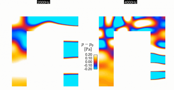
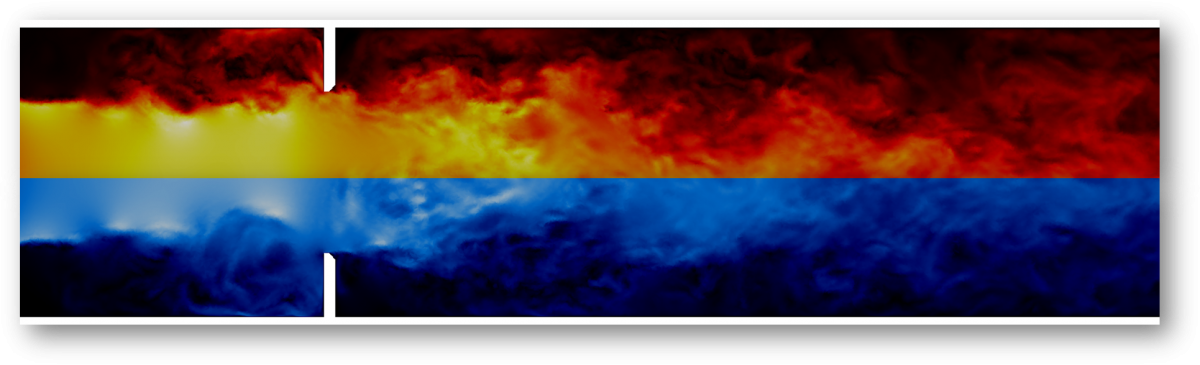
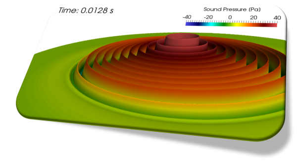
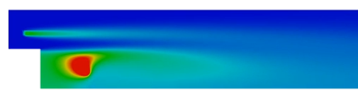
The reflection at the boundary has a larger effect on the solution especially when we perform a compressible flow simulation as can be seen in the following movie (Upper: With reflection, Lower: Without reflection of sound wave).

In OpenFOAM, we can use two approximate non-reflecting boundary conditions:

They determine the boundary value by solving the following equation

\begin{align}
\frac{D \phi}{D t} = \frac{\partial \phi}{\partial t} + \boldsymbol{U} \cdot \nabla \phi = 0, \tag{1} \label{eq:advection}
\end{align}

where \(D/Dt\) is the material derivative and \(\boldsymbol{U}(\boldsymbol{x}, t)\) is the advection velocity.

We assume that the advection velocity \(\boldsymbol{U}\) is parallel to the boundary (face) normal direction and rewrite the eqn. \eqref{eq:advection} as

\begin{align}
\frac{D \phi}{Dt} \approx \frac{\partial \phi}{\partial t} + U_{n} \cdot \frac{\partial \phi}{\partial \boldsymbol{n}}= 0, \tag{2} \label{eq:advection2}
\end{align}

where \(\boldsymbol{n}\) is the outward-pointing unit normal vector.

These boundary conditions are different in how the advection speed (scalar quantity) \(U_{n}\) is calculated and it is calculated in advectionSpeed() member function.

advective B.C.

The advection speed is the component of the velocity normal to the boundary

\begin{align}
U_n = u_n. \tag{3} \label{eq:advectiveUn}
\end{align}

waveTransmissive B.C.

The advection speed is the sum of the component of the velocity normal to the boundary and the speed of sound \(c\)

\begin{align}
U_n = u_n + c = u_n + \sqrt{\gamma/\psi}, \tag{4} \label{eq:waveTransmissiveUn}
\end{align}

where \(\gamma\) is the ratio of specific heats \(C_p/C_v\) and \(\psi\) is compressibility.

What do lInf and fieldInf mean?

Coming soon.

Numerical Libraries – Linear Algebra

This page will be sequentially updated.

The linear algebraic operations, such as solving systems of linear equations and matrix multiplication, often appear in the field of machine learning, computational fluid dynamics, computer graphics, and so on. As the dimensions of systems or matrices will be bigger, these operations will become more time consuming and complicated.

There are many optimized open-source numerical libraries for linear algebra, such as LAPACK and Eigen, so we can use them to get better performance even when our matrices are very large.

For example, an open source CFD software SU2 uses BLAS and LAPACK, and moreover the performance of NumPy can be improved with the use of these optimized linear algebra libraries.

In this page, I try to succinctly summarize what we need to know at a minimum about open-source numerical libraries.

BLAS (Basic Linear Algebra Subprograms)
  • [URL] http://www.netlib.org/blas/
  • BLAS libraries provide standard building blocks for performing basic vector and matrix operations
    • Level 1: scalar, vector and vector-vector operations
    • Level 2: matrix-vector operations
    • Level 3: matrix-matrix operations
BLACS (Basic Linear Algebra Communication Subprograms)
LAPACK (Linear Algebra PACKage)
ScaLAPACK (Scalable Linear Algebra PACKage)
Eigen

Finite Difference Time Domain (FDTD) Method


The Finite Difference Time Domain (FDTD) method was originally developed by K. S. Yee in 1966 as a numerical technique to solve Maxwell’s equations in time domain. As the name implies, the FDTD method is based on the finite difference approximation to discretize partial differential equations.

The ideas of the FDTD method have been applied to other wave-field phenomena. For example, Madariga introduced the FDTD method in elastodynamics in 1976 and it is currently used in acoustic field analysis to solve sound wave propagation in time and space.

Acoustics simulation techniques

We’ll start a 10-part series of blog posts about applications of the FDTD in acoustic field analysis.

  • Governing equations
  • Boundary Conditions: Rigid body
  • Boundary Conditions: Sound absorbing boundary
  • Perfectly Matched Layer (PML)
  • Sound source
  • Scattering
  • Diffraction
  • Interference
  • Resonance
  • Refraction

Diffusion Term of the N-S Equations Part1


The mathematical expressions of the viscous stress differ between Newtonian fluids and non-Newtonian fluids, so do those of the diffusion term. In this post, we consider only Newtonian fluids, such as air and water.

Many turbulence models treat the effects of the turbulence as augmentation of mixing or diffusion, but the modeled expression differs depending on the turbulence models, such as linear eddy-viscosity, non-linear eddy viscosity and Reynolds-stress transport models.

We’ll start by running through mathematical expressions of the diffusion term and find out how these are implemented in OpenFOAM.

Diffusion term (Newtonian fluids)

For Newtonian fluids the ratio of the shear stress to the shear rate is constant and the diffusion term of the Navier-Stokes equations are given by:

\begin{equation}
\nabla \cdot \left( \mu \left( \nabla \boldsymbol{u} + (\nabla \boldsymbol{u})^T \right) -\frac{2}{3}\mu (\nabla \cdot \boldsymbol{u}) \boldsymbol{I} \right), \tag{1} \label{eq:newtondiffusion}
\end{equation}
where \(\boldsymbol{u}\) is the velocity field, \(\mu\) is the molecular viscosity and \(\boldsymbol{I}\) is the identity tensor.

In the case of laminar flows and Direct Numerical Simulations (DNS) of turbulent flows, this expression is used.

When we solve turbulent flows with turbulence models, the expression of the diffusion term changes from Eq. \eqref{eq:newtondiffusion} according to the model we choose. If we use the linear eddy-viscosity models of Reynolds-averaged Navier-Stokes (RANS), such as k-\(\epsilon\) and k-\(\omega\) SST models, the Reynolds stress is modeled with the following expression:

\begin{equation}
-\rho\overline{\boldsymbol{u}\boldsymbol{u}} = \mu_t \left( \nabla \overline{\boldsymbol{u}} + (\nabla \overline{\boldsymbol{u}})^T \right) -\frac{2}{3}\rho k \boldsymbol{I}, \tag{2} \label{eq:BoussinesqApprox}
\end{equation}

and the diffusion term is expressed as:

\begin{align}
&\nabla \cdot \left( \mu \left( \nabla \overline{\boldsymbol{u}} + (\nabla \overline{\boldsymbol{u}})^T \right) -\frac{2}{3}\mu (\nabla \cdot \overline{\boldsymbol{u}}) \boldsymbol{I} -\rho\overline{\boldsymbol{u}\boldsymbol{u}} \right) \\
=& \nabla \cdot \left( (\mu + \mu_t) \left( \nabla \overline{\boldsymbol{u}} + (\nabla \overline{\boldsymbol{u}})^T \right) -\frac{2}{3}\mu (\nabla \cdot \overline{\boldsymbol{u}}) \boldsymbol{I} – \frac{2}{3}\rho k \boldsymbol{I} \right) \\
=& \nabla \cdot \left( \mu_{eff} \left( \nabla \overline{\boldsymbol{u}} + (\nabla \overline{\boldsymbol{u}})^T \right) -\frac{2}{3}\mu (\nabla \cdot \overline{\boldsymbol{u}}) \boldsymbol{I} \right) – \nabla \cdot \left( \frac{2}{3}\rho k \boldsymbol{I} \right), \tag{3} \label{eq:levmdiffusion}
\end{align}
where \(\overline{\boldsymbol{u}}\) is the ensemble-averaged velocity field, \(k\) is the turbulence energy, \(\rho\) is the density and the effective viscosity \(\mu_{eff}\) is the sum of the molecular and turbulent eddy viscosity \(\mu_t\).

If the flow is incompressible, the expression reduces to the following one because of the continuity equation \(\nabla \cdot \overline{\boldsymbol{u}} = 0\):
\begin{equation}
\nabla \cdot \left( \mu_{eff} \left( \nabla \overline{\boldsymbol{u}} + (\nabla \overline{\boldsymbol{u}})^T \right) \right) – \nabla \cdot \left( \frac{2}{3}\rho k \boldsymbol{I} \right). \tag{4} \label{eq:incompdiffusion}
\end{equation}

If turbulence models of the eddy-viscosity type is used, the effects of fluctuating turbulent flows are expressed as augmentation of the diffusion as can be seen from Eq. \eqref{eq:levmdiffusion}.

We are all set!
Let’s look into how the diffusion term is handled in OpenFOAM 🙂

Implementation in OpenFOAM

If we have a quick look at UEqn.H file of rhoPimpleFoam, a transient compressible flow solver, we can find turbulence->divDevRhoReff(U) in it. It corresponds to the diffusion term.

We can find its definitions in different files depending on the types of the turbulence models. In the case of linear eddy viscosity models, it is defined in linearViscousStress.C file.

We can find a tiny difference by comparing it with Eq. \eqref{eq:levmdiffusion}:
l.10
\begin{equation}
\nabla \cdot \left( \mu_{eff} \left( (\nabla \overline{\boldsymbol{u}})^T -\frac{2}{3} (\nabla \cdot \overline{\boldsymbol{u}}) \boldsymbol{I} \right) \right), \tag{5} \label{eq:levmdiffusion1}
\end{equation}
l.11
\begin{equation}
\nabla \cdot \left( \mu_{eff} \nabla \overline{\boldsymbol{u}} \right). \tag{6} \label{eq:levmdiffusion2}
\end{equation}

The remaining term \(- \nabla \cdot \left( \frac{2}{3}\rho k \boldsymbol{I} \right)\) is included in the pressure gradient term.

In the next post, we’ll look into non-linear eddy viscosity models and Reynolds-stress transport models.

Thank you for taking the time to read all of my post!

[May 4, 2019] Notices from the blog

Please let us know your opinion if you have any suggestions to make this blog even better for both of us!

[May 4, 2019] Contact Form

Contact form is now available at the bottom of each page. Please feel free to contact us if you have any requests for the topics to be covered on the blog.

[May 1, 2019] Always-On SSL

We have enhanced security of our entire website by applying Always-On SSL (AOSSL). Accordingly, our website address has changed to the following URL:

[Old] http://caefn.com
[New] https://caefn.com

Our old URL will be automatically redirected to the new one, but please be sure to update any bookmarks or favorites you may have registered.

Turbulence Models in OpenFOAM – Hybrid Methods

Last Updated: May 4, 2019

Large Eddy Simulation (LES) can be used to accurately simulate unsteady flow behaviors but its numerical cost is higher compared to the conventional Reynolds Averaged Navier-Stokes (RANS) approach.

Several methods have been developed in order to save computational time and cost for unsteady flow computations compared to LES.

Keywords
Detached-Eddy Simulation (DES), Scale Adaptive Simulation (SAS), Grey area problem

Detached Eddy Simulation (DES)

Detached-Eddy Simulation (DES) is a hybrid Reynolds Averaged Navier-Stokes/Large-Eddy Simulation model. The DES model was first proposed in 1997 by Spalart et al. [1] based on the Spalart-Allmaras RANS model and it is commonly referred to as DES97.

Spalart-Allmaras Based DES Formulation (DES97)

Its formulation is briefly described in [2]:

The driving length scale of the RANS S-A model is the distance to the closest wall, \(d\). This makes a modification to this model for DES mode quite straightforward (exactly for this reason it was used as a basis of DES in the first publication [1]). The modification consists in substituting for \(d\), everywhere in the equations, the new DES length scale, \(\tilde{d}\). This length is also based on the grid spacing \(\Delta\) and is defined as:
\begin{equation}
\tilde{d} = {\rm min}\left( d, C_{DES}\Delta \right), \tag{1} \label{eq:dTilda}
\end{equation}
where \(C_{DES}\) is the only new adjustable model constant, and \(\Delta\) is based on the largest dimension of the local grid cell
\begin{equation}
\Delta = {\rm max}\left( \delta_{x}, \delta_{y}, \delta_{z} \right). \tag{2} \label{eq:delta}
\end{equation}
Here we assume for simplicity that the grid is structured and that the coordinates \(\left(x, y, z\right)\) are aligned with the grid cell, but the generalizations are obvious.

For wall-bounded separated flows, the above formulation results in a bybrid model that functions as the standard RANS S-A model inside the whole attached boundary layer, and as its subgrid-scale version in the rest of the flow including the separated regions and near wake. Indeed, in the attached boundary layer, due to the significant grid anisotropy \(\left(\delta_{x} \approx \delta_{z} \gg \delta_{y}\right)\) typical of this flow region, in accordance with \eqref{eq:dTilda}, \(\tilde{d} = d\), and the model reduces to the standard S-A RANS model. Otherwise, once a field point is far enough from walls \(\left( d > C_{DES}\Delta \right)\), the length scale of the model becomes grid-dependent, i.e., the model performs as a subgrid-scale version of the S-A model. Note that at “equilibrium” (meaning a balance of production and destruction terms) this model reduces to an algebraic miximg-length Smagorinski-like subgrid model.

The “DES limiter” defined by Eq. \eqref{eq:dTilda} that is used in DES97 switches between the RANS length scale and LES length scale so that the model behaves in RANS-like and LES-like manners as illustrated in Figure 1. The length scale \eqref{eq:dTilda} depends only on the grid used in the simulation and it is solution-independent.

Figure 1: Schematic illustration of S-A based DES model.

Menter’s SST Based DES Formulation

  • k-\(\omega\) SST DES model
  • k-\(\omega\) SST DDES model
  • k-\(\omega\) SST IDDES model

There is a project called DESider (Detached Eddy Simulation for Industrial Aerodynamics) and many other DES models have been developed based on different RANS models, including RSM ones.

Other Models

  • \(v^2-f\) DES model

We can check the RANS and LES regions using the DESModelRegions function objects in OpenFOAM.

Scale Adaptive Simulation (SAS)
  • k-\(\omega\) SST SAS model
Useful Links
  • FLOMANIA (Flow Physics Modelling An Integrated Approach) Project: 2002-2004
  • DESider (Detached Eddy Simulation for Industrial Aerodynamics) Project: 2004-2007
  • ATAAC (Advanced Turbulence Simulation for Aerodynamic Application Challenges) Project
References

[1] P. R. Spalart, W.-H. Jou, M. Strelets and S. R. Allmaras, Comments on the feasibility of LES for wings, and on a hybrid RANS/LES approach. 1st AFOSR Int. Conf. on DNS/LES, Aug. 4-8, 1997, Ruston, LA. In “Advances in DNS/LES”, C. Liu and Z. Liu Eds., Greyden Press, Columbus, OH.
[2] M. Strelets, Detached Eddy Simulation of Massively Separated Flows. AIAA, 2001-0879.
[3] P. R. Spalart, S. Deck, M. L. Shur, K. D. Squires, M. Kh. Strelets, and A. Travin, A new version of detached-eddy simulation, resistant to ambiguous grid densities. Theoretical and Computational Fluid Dynamics, 20(3), 181-195, 2006.
[4] M. L. Shur, P. R. Spalart, M. Kh. Strelets, and A. Travin, A hybrid RANS-LES approach with delayed-DES and wall-modelled LES capabilities. International Journal of Heat and Fluid Flow, 29, 1638–1648, 2008.
[5] Detached eddy simulation (DES). Available at: http://www.cfd-online.com/Wiki/Detached_eddy_simulation_(DES) [Accessed: 03 May 2019].
[6] OpenFOAM® v3.0+: New Solver and Physical Modelling Functionality. Available at: https://www.openfoam.com/releases/openfoam-v3.0+/solvers-and-physics.php#physics-kOmegaSSTDES [Accessed: 03 May 2019].
[7] C. M. Winkler, A. J. Dorgan and M. Mani, Scale Adaptive Simulations of Turbulent Flows on Unstructured Grids. AIAA, 2011-3559.

fvOptions acousticDampingSource

Last Updated: May 3, 2019

For accurate computational aeroacoustics (CAA) simulations, we have to prevent the acoustic waves from reflecting on the truncated boundary of the computational domain so that the reflected waves will not contaminate the acoustic field by wave interference.

A variety of numerical techniques have been developed for this purpose. In this blog post, I will try to give a description of one of these methods, namely the artificial damping (dissipation) method.

General Description

This damping method is briefly described in [1].

In this method, an absorbing zone is created and appended to the physical computational domain in which the governing equations are modified to mimic a physical dissipation mechanism.

For the Euler and Navier-Stokes equations, the artificial damping term can easily be introduced into the governing equations as follows:

\begin{align}
\frac{\partial \boldsymbol{u}}{\partial t} = L(\boldsymbol{u})\; – \nu(\boldsymbol{u} – \boldsymbol{u}_0), \tag{5.155} \label{eq:damping}
\end{align}

where \(\boldsymbol{u}\) is the solution vector and \(L(\boldsymbol{u})\) denotes the spatial operators of the equations. The damping coefficient \(\nu\) assumes a positive value and should be increased slowly inside the zone. Here, \(\boldsymbol{u}_0\) is the time-independent mean value in the absorbing zone (Freund 1997). Kosloff and Kosloff (1986) analyzed a system similar to Equation \eqref{eq:damping} for the two-dimensional wave equation in which, in particular, a reflection coefficient of a multilayer absorbing zone was calculated.

The role of the artificial damping term is to diminish the strength of the waves in the absorbing zone before they reach the truncated boundary and to minimize the reflecting effect.

acousticdampingsource2

Settings of acousticDampingSource

In OpenFOAM v1606+, this artificial damping method is available as the newly implemented fvOption acousticDampingSource [2]. Its settings are described in the system/fvOptions file.

  • timeStart: [Optional] Start time
  • duration: [Optional] Duration time
  • selectionMode: [Required] Domain where the source is applied (all/cellSet/cellZone/points)
  • centre: [Required] Sphere centre location of damping
  • radius1: [Required] Inner radius at which to start damping
  • radius2: [Required] Outer radius beyond which full damping is applied
  • frequency: [Required] Frequency [Hz]
  • w: [Optional] Stencil width (default = 20)
  • Uref: [Required] Name of reference velocity field

The strength of damping is gradually increased from radius1 to radius2 and full damping is applied in the region where \(r >\) radius2. The maximum value of damping coefficient is defined as follows:

\begin{align}
\nu_{max} = w \times frequency. \tag{1} \label{eq:maxnu}
\end{align}

acousticdampingsource3

This function is only applicable for the momentum equation by default, so it needs source modifications so that it can be used in the mass and energy conservation equations as well.

An Example in 1D (Plane Wave)

Sound waves are longitudinal waves but I intentionally visualize them like the transverse waves in order to make the damping effect more visible in the following video. The damping is activated at time = 0.004s.

An Example in 2D (Cylindrical Wave)

Sound waves are longitudinal waves but I intentionally visualize them like the transverse waves in order to make the damping effect more visible in the following video. The damping is activated at time = 0.004s.

The amplitude gets smaller as they propagate from a sound source in contrast to the plane waves (cylindrical spreading).

Aeolian Tone

aeoliantone

Source Code

The damping source terms added to the incompressible and compressible momentum equations are calculated by Eq. \eqref{eq:damping} in addSup function.

The profile of damping coefficient in the radial direction is calculated by the trigonometric (cosine) function in setBlendingFactor helper function.

References
  • [1] Claus Albrecht Wagner et al., Large-Eddy Simulation for Acoustics (Cambridge Aerospace Series)
  • [2] OpenFOAM® v1606+: New Solvers. Available at: https://www.openfoam.com/releases/openfoam-v1606+/solvers-and-physics.php#solvers-and-physics-acoustic-damping [Accessed: 03 May 2019].

fvOptions SemiImplicitSource

Last Updated: May 5, 2019

When we solve a partial differential equation with a source term, we must pay attention to how to treat it numerically for better convergence. The SemiImplicitSource fvOption is available in OpenFOAM so that we can handle a linearized source term in numerically stable way.

Keywords

  • Source term linearization
  • SemiImplicitSource in OpenFOAM
Source Term Linearization

If the source term under consideration is a non-linear function of a conserved variable, the linearization of it is a fundamental approach to discretizing it in the finite volume method. This topic is precisely covered in the famous book “Numerical Heat Transfer and Fluid Flow” by Suhas V. Patankar:

In Section 4.2.5, the concept of the linearization of the source term was introduced. One of the basic rules (Rule 3) required that when the source term is linearized as

\begin{equation}
S = S_C + S_P \phi_P, \tag{7.6} \label{eq:sourceTerm}
\end{equation}

the quantity \(S_P\) must not be positive. Now, we return to the topic of source-term linearization to emphasize that often source terms are the cause of divergence of iterations and that proper linearization of the source term frequently holds the key to the attainment of a converged solution.

Rule 3: Negative-slope linearization of the source term If we consider the coefficient definitions in Eqs. (3.18), it appears that, even if the neighbor coefficients are positive, the center-point coefficient \(a_P\) can become negative via the \(S_P\) term. Of course, the danger can be completely avoided by requiring that \(S_P\) will not be positive. Thus, we formulate Rule 3 as follows:

When the source term is linearized as \(\bar{S} = S_C + S_P T_P\), the coefficient \(S_P\) must always be less than or equal to zero.

Linearized Source Specification for a Scalar Field in OpenFOAM

In OpenFOAM, the linearized source terms can be specified using SemiImplicitSource fvOption. Its settings are described in the constant/fvOptions file.

  • selectionMode: [Required] Domain where the source is applied (all/cellSet/cellZone/points)
  • injectionRateSuSp: [Required] Conserved variable name and two coefficients of linearized source term

  • volumemode: [Required] Choice of how to specify the two coefficients

absolute: values are given as [variable]

specific: values are given as [variable]/\({\rm m^3}\)

Example 1. Heat Conduction with Heat Source

Let’s consider a simple 1D heat conduction problem in a solid rod with a thermal energy generation per unit volume and time \(\dot{q}_v {\rm [W/m^3]}\). In this case, the steady heat conduction equation in 1D is given by

\begin{align}
\alpha \frac{d^2 T}{d x^2} + \frac{\dot{q}_v}{\rho c} = 0. \tag{1} \label{eq:conductionEqn}
\end{align}

Here, we assume that the thermal diffusivity \(\alpha {\rm [m^2/s]}\) is constant.

We can obtain the general solution for this equation \eqref{eq:conductionEqn} by integrating it twice.

\begin{equation}
T(x) = -\frac{S_C}{2\alpha}x^2 + C_1 x + C_2, \tag{2} \label{eq:generalSolution}
\end{equation}

where \(C_1\) and \(C_2\) are integration constants and we put \(S_C {\rm [K/s]} := \dot{q}_v/\rho c\). If we assume that the temperatures at both ends of the rod are maintained at constant temperatures \(T(0) = T_1, T(L) = T_2\), we can determine the values of two integration constants as

\begin{align}
C_2 &= T_1, \tag{3} \\
C_1 &= \frac{T_2 – T_1}{L} + \frac{S_C L}{2\alpha}. \tag{4}
\end{align}

Then, the temperature distribution in the rod is expressed by the following equation:

\begin{equation}
T(x) = -\frac{S_C}{2\alpha}x^2 + \left( \frac{T_2 – T_1}{L} + \frac{S_C L}{2\alpha} \right)x + T_1. \tag{5} \label{eq:solution}
\end{equation}

t_heatsource_case1

t_heatsource

If we confine the heat source region to one-quarter of the whole region as shown in the following picture, the quadratic temperature distribution is limited to the region and the linear profile is obtained in the source free region.

t_heatsource_case2_ps2

t_heatsource_case2

t_heatsource_case2b

Example 2. Passive Scalar Transport