\(\rho_{l,Sat}\):
\(\rho_{v,Sat}\):
\(\psi_{l} \times 10^7\):
\(\psi_{v} \times 10^7\):
\(\rho_{v,Sat}\):
\(\psi_{l} \times 10^7\):
\(\psi_{v} \times 10^7\):
Open The Way To Customizations
I will implement some calculators to estimate the proper settings for the boundary prism layer meshing.
Simple mathematical calculations, such as the four arithmetic operations and power, can be done using HTML and JavaScript.
\begin{align}
l_{n} = l_{1} r^{n-1}
\end{align}
\begin{align}
l_{tot} = \sum_{k=1}^{n} l_{1} r^{k-1} = \frac{l_{1} \left( r^n – 1 \right)}{r – 1} \left( r \neq 1 \right)
\end{align}
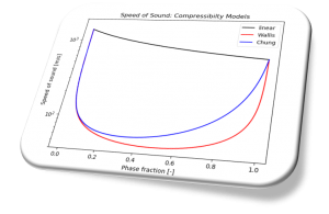
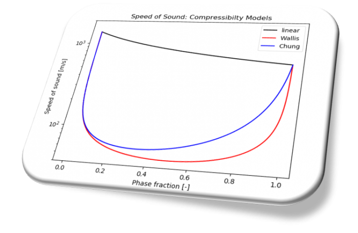
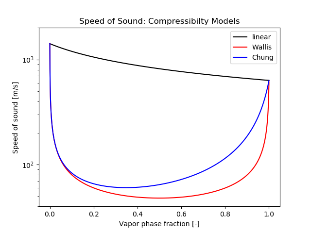
We want to plot the following three mathematical expressions in 2D that describe the speed of sound \(c\) as a function of a vapor fraction \(\gamma\).
\begin{align}
c = \frac{1}{\sqrt{\psi}}. \tag{1} \label{eq:psi-sos}
\end{align}
\begin{align}
\psi_{linear} = \gamma \psi_v + \left(1 – \gamma \right)\psi_l \tag{2} \label{eq:linear}
\end{align}
\begin{align}
\psi_{Wallis} = \left( \gamma \rho_{v, Sat} + \left( 1 – \gamma \right)\rho_{l, Sat} \right)
\left( \gamma \frac{\psi_v}{\rho_{v, Sat}} + \left( 1 – \gamma \right)\frac{\psi_l}{\rho_{l, Sat}} \right) \tag{3} \label{eq:wallis}
\end{align}
\begin{align}
\psi_{Chung} = \left( \left( \frac{1 – \gamma}{\sqrt{\psi_v}} + \gamma \frac{s_{fa}}{\sqrt{\psi_l}} \right)\frac{\sqrt{\psi_v \psi_l}}{s_{fa}} \right)^2 \tag{4} \label{eq:chung}
\end{align}
where
\begin{align}
s_{fa} = \sqrt{ \frac{\frac{\rho_{v, Sat}}{\psi_v}}{\left( 1- \gamma \right)\frac{\rho_{v, Sat}}{\psi_v} + \gamma \frac{\rho_{l, Sat}}{\psi_l}} } \tag{5} \label{eq:chung-sfa}
\end{align}
For more details of the above expressions, you might want to read the following post.
|
1 2 3 4 5 6 7 8 9 10 11 12 13 14 15 16 17 18 19 20 21 22 23 24 25 26 27 28 29 30 31 32 33 34 |
import matplotlib.pyplot as plt import numpy as np # linear compressibility model def psi_linear(x): return x*psiv + (1 - x)*psil # Wallis compressibility model def psi_wallis(x): return (x*rhovsat + (1 - x)*rholsat)*(x*psiv/rhovsat + (1 - x)*psil/rholsat) # Chung compressibility model def psi_chung(x): sfa = np.sqrt((rhovsat/psiv)/((1 - x)*rhovsat/psiv + x*rholsat/psil)) return np.square(((1 - x)/np.sqrt(psiv) + x*sfa/np.sqrt(psil))*np.sqrt(psiv*psil)/sfa) # User inputs psiv = 2.5e-06 psil = 5.0e-07 rhovsat = 1.2 rholsat = 830 gamma = np.arange(0, 1, 1e-04) plt.title('Speed of Sound: Compressibilty Models') plt.xlabel('Vapor phase fraction [-]') plt.ylabel('Speed of sound [m/s]') plt.ylim(40, 2000) plt.yscale('log') plt.plot(gamma, 1/np.sqrt(psi_linear(gamma)), color="black", linewidth=1.5, label='linear') plt.plot(gamma, 1/np.sqrt(psi_wallis(gamma)), color="red", linewidth=1.5, label='Wallis') plt.plot(gamma, 1/np.sqrt(psi_chung(gamma)), color="blue", linewidth=1.5, label='Chung') plt.legend(loc='best') plt.show() |
The famous physics textbook written by the theoretical physicist L. D. Landau and E. M. Lifshitz are freely accessible from the following links.
https://archive.org/details/Mechanics3eLandauLifshitz
https://archive.org/details/TheClassicalTheoryOfFields
https://archive.org/details/QuantumMechanics_104
https://archive.org/details/RelativisticQuantumTheoryPart1
https://archive.org/details/ost-physics-landaulifshitz-statisticalphysics
https://archive.org/details/FluidMechanics
https://archive.org/details/TheoryOfElasticity
https://archive.org/details/ElectrodynamicsOfContinuousMedia
Last Updated: June 9, 2019
The cavitatingFoam is a transient cavitation solver based on the homogeneous equilibrium model (HEM) from which the compressibility of the liquid/vapour ‘mixture’ is obtained, whose density varies from liquid density to vapor one according to the chosen barotropic equation of state.
\begin{align}
\frac{D \rho}{Dt} = \psi \frac{Dp}{Dt} \tag{1} \label{eq:eos}
\end{align}
\begin{align}
\psi = \rho \beta_s \tag{2} \label{eq:psi}
\end{align}
The definition of the isentropic compressibility can be deformed in the following way:
\begin{align}
\beta_s &\equiv -\frac{1}{V} \left( \frac{\partial V}{\partial p} \right)_s \tag{3} \label{eq:betas} \\
&= -\frac{1}{V} \left(\frac{\partial V}{\partial \rho} \frac{\partial \rho}{\partial p} \right)_s \\
&= \rho \frac{1}{\rho^2} \left(\frac{\partial \rho}{\partial p} \right)_s \\
&= \frac{1}{\rho c^2}
\end{align}
where \(c\) is the speed of sound. We can substitute this expression for \(\beta_s\) in \eqref{eq:psi}, obtaining the following expression:
\begin{align}
\psi = \frac{1}{c^2}. \tag{4} \label{eq:psi-sos}
\end{align}
The compressibility of the mixture equals to the reciprocal of the square of the speed of sound.
We can specify a compressibility function \(\psi\) that defines the coupling between the density and pressure in the thermophysicalProperties file.
The following three models for \(\psi\) are available in OpenFOAM v1812.
|
1 2 3 4 5 6 7 8 9 10 11 12 13 14 15 16 17 18 19 20 21 22 23 24 25 26 27 28 29 30 |
/*--------------------------------*- C++ -*----------------------------------*\ | ========= | | | \\ / F ield | OpenFOAM: The Open Source CFD Toolbox | | \\ / O peration | Version: v1812 | | \\ / A nd | Web: www.OpenFOAM.com | | \\/ M anipulation | | \*---------------------------------------------------------------------------*/ FoamFile { version 2.0; format ascii; class dictionary; location "constant"; object thermodynamicProperties; } // * * * * * * * * * * * * * * * * * * * * * * * * * * * * * * * * * * * * * // barotropicCompressibilityModel linear; psiv 2.5e-06; rholSat 830; psil 5e-07; pSat 4500; rhoMin 0.001; // ************************************************************************* // |
The expressions of the speed of sound \(c\) in the liquid/vapour mixture are different according to the selected function.

\begin{align}
\psi = \gamma \psi_v + \left(1 – \gamma \right)\psi_l \tag{5} \label{eq:linear}
\end{align}
|
75 76 77 78 |
void Foam::compressibilityModels::linear::correct() { psi_ = gamma_*psiv_ + (scalar(1) - gamma_)*psil_; } |
\begin{align}
s_{fa} = \sqrt{ \frac{\frac{\rho_{v, Sat}}{\psi_v}}{\left( 1- \gamma \right)\frac{\rho_{v, Sat}}{\psi_v} + \gamma \frac{\rho_{l, Sat}}{\psi_l}} } \tag{6} \label{eq:chung-sfa}
\end{align}
\begin{align}
\psi = \left( \left( \frac{1 – \gamma}{\sqrt{\psi_v}} + \gamma \frac{s_{fa}}{\sqrt{\psi_l}} \right)\frac{\sqrt{\psi_v \psi_l}}{s_{fa}} \right)^2 \tag{7} \label{eq:chung}
\end{align}
|
86 87 88 89 90 91 92 93 94 95 96 97 98 99 100 101 102 |
void Foam::compressibilityModels::Chung::correct() { volScalarField sfa ( sqrt ( (rhovSat_/psiv_) /((scalar(1) - gamma_)*rhovSat_/psiv_ + gamma_*rholSat_/psil_) ) ); psi_ = sqr ( ((scalar(1) - gamma_)/sqrt(psiv_) + gamma_*sfa/sqrt(psil_)) *sqrt(psiv_*psil_)/sfa ); } |
\begin{align}
\psi = \left( \gamma \rho_{v, Sat} + \left( 1 – \gamma \right)\rho_{l, Sat} \right)
\left( \gamma \frac{\psi_v}{\rho_{v, Sat}} + \left( 1 – \gamma \right)\frac{\psi_l}{\rho_{l, Sat}} \right) \tag{8} \label{eq:wallis}
\end{align}
\begin{align}
\frac{\psi}{\gamma \rho_{v, Sat} + \left( 1 – \gamma \right)\rho_{l, Sat}} = \gamma \frac{\psi_v}{\rho_{v, Sat}} + \left( 1 – \gamma \right)\frac{\psi_l}{\rho_{l, Sat}} \tag{8′} \label{eq:wallis2}
\end{align}
|
86 87 88 89 90 91 |
void Foam::compressibilityModels::Wallis::correct() { psi_ = (gamma_*rhovSat_ + (scalar(1) - gamma_)*rholSat_) *(gamma_*psiv_/rhovSat_ + (scalar(1) - gamma_)*psil_/rholSat_); } |
[1] Christopher Earls Brennen, Fundamentals of Multiphase Flow. Cambridge University Press (2005)
Constant dispersed-phase particle diameter model.
|
1 2 3 4 5 6 7 8 9 10 |
water { diameterModel constant; constantCoeffs { d 1e-4; } residualAlpha 1e-6; } |
|
68 69 70 71 72 73 74 75 76 77 78 79 80 81 82 83 84 85 86 87 |
Foam::tmp<Foam::volScalarField> Foam::diameterModels::constant::d() const { return tmp<Foam::volScalarField> ( new volScalarField ( IOobject ( "d", phase_.U().time().timeName(), phase_.U().mesh(), IOobject::NO_READ, IOobject::NO_WRITE, false ), phase_.U().mesh(), d_ ) ); } |
Isothermal dispersed-phase particle diameter model.
\begin{align}
p \times \frac{4}{3} \pi \left( \frac{d}{2} \right)^3 &= p_0 \times \frac{4}{3} \pi \left( \frac{d_0}{2} \right)^3 \\
d &= d_0 \left( \frac{p_0}{p} \right)^{1/3} \tag{1} \label{eq:levmdiffusion}
\end{align}
|
1 2 3 4 5 6 7 8 9 10 11 |
air { diameterModel isothermal; isothermalCoeffs { d0 3e-3; p0 1e5; } residualAlpha 1e-6; } |
|
69 70 71 72 73 74 75 76 77 |
Foam::tmp<Foam::volScalarField> Foam::diameterModels::isothermal::d() const { const volScalarField& p = phase_.U().db().lookupObject<volScalarField> ( "p" ); return d0_*cbrt(p0_/p); } |
IATE (Interfacial Area Transport Equation) bubble diameter model.
Solves for the interfacial curvature per unit volume of the phase rather than interfacial area per unit volume to avoid stability issues relating to the consistency requirements between the phase fraction and interfacial area per unit volume.
|
1 2 3 4 5 6 7 8 9 10 11 12 13 14 15 16 17 18 19 20 21 22 23 24 25 26 27 28 29 30 31 32 |
air { diameterModel IATE; IATECoeffs { dMax 1e-2; dMin 1e-4; residualAlpha 1e-6; sources ( wakeEntrainmentCoalescence { Cwe 0.002; } randomCoalescence { Crc 0.04; C 3; alphaMax 0.75; } turbulentBreakUp { Cti 0.085; WeCr 6; } ); } residualAlpha 1e-6; } |
The following bubble interaction mechanisms are considered in this model.
|
115 116 117 118 119 120 121 122 123 124 125 126 127 128 129 130 131 132 133 134 135 136 137 138 139 140 141 142 143 144 145 146 147 148 149 150 151 152 153 154 155 156 157 158 159 160 161 162 163 |
Foam::tmp<Foam::volScalarField> Foam::diameterModels::IATE::dsm() const { return max(6/max(kappai_, 6/dMax_), dMin_); } void Foam::diameterModels::IATE::correct() { // Initialise the accumulated source term to the dilatation effect volScalarField R ( ( (1.0/3.0) /max ( fvc::average(phase_ + phase_.oldTime()), residualAlpha_ ) ) *(fvc::ddt(phase_) + fvc::div(phase_.alphaPhi())) ); // Accumulate the run-time selectable sources forAll(sources_, j) { R -= sources_[j].R(); } fv::options& fvOptions(fv::options::New(phase_.mesh())); // Construct the interfacial curvature equation fvScalarMatrix kappaiEqn ( fvm::ddt(kappai_) + fvm::div(phase_.phi(), kappai_) - fvm::Sp(fvc::div(phase_.phi()), kappai_) == - fvm::SuSp(R, kappai_) //+ Rph() // Omit the nucleation/condensation term + fvOptions(kappai_) ); kappaiEqn.relax(); fvOptions.constrain(kappaiEqn); kappaiEqn.solve(); // Update the Sauter-mean diameter d_ = dsm(); } |
In this page, I will organize information on the physical models available in twoPhaseEulerFoam, an Eulerian-Eulerian solver available in OpenFOAM.
I will add descriptions of each model.
Selected OpenFOAM version: