cavitatingFoam – barotropicCompressibilityModel (v1812)

Last Updated: June 9, 2019

The cavitatingFoam is a transient cavitation solver based on the homogeneous equilibrium model (HEM) from which the compressibility of the liquid/vapour ‘mixture’ is obtained, whose density varies from liquid density to vapor one according to the chosen barotropic equation of state.

Compressibility and speed of sound

\begin{align}
\frac{D \rho}{Dt} = \psi \frac{Dp}{Dt} \tag{1} \label{eq:eos}
\end{align}

\begin{align}
\psi = \rho \beta_s \tag{2} \label{eq:psi}
\end{align}

  • \(\rho\): density
  • \(p\): pressure
  • \(\beta_s\): isentropic compressibility

The definition of the isentropic compressibility can be deformed in the following way:
\begin{align}
\beta_s &\equiv -\frac{1}{V} \left( \frac{\partial V}{\partial p} \right)_s \tag{3} \label{eq:betas} \\
&= -\frac{1}{V} \left(\frac{\partial V}{\partial \rho} \frac{\partial \rho}{\partial p} \right)_s \\
&= \rho \frac{1}{\rho^2} \left(\frac{\partial \rho}{\partial p} \right)_s \\
&= \frac{1}{\rho c^2}
\end{align}
where \(c\) is the speed of sound. We can substitute this expression for \(\beta_s\) in \eqref{eq:psi}, obtaining the following expression:
\begin{align}
\psi = \frac{1}{c^2}. \tag{4} \label{eq:psi-sos}
\end{align}
The compressibility of the mixture equals to the reciprocal of the square of the speed of sound.

We can specify a compressibility function \(\psi\) that defines the coupling between the density and pressure in the thermophysicalProperties file.

barotropicCompressibilityModel

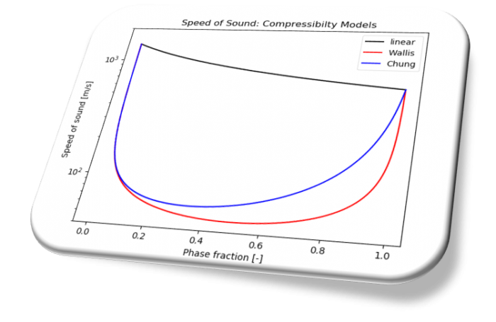
The following three models for \(\psi\) are available in OpenFOAM v1812.

  • linear
  • Chung
  • Wallis

  • psiv: compressibility \(\psi\) of the vapor phase
  • psil: compressibility \(\psi\) of the liquid phase
  • pSat: saturation pressure
  • rhovSat: density of vapor at saturation point
  • rholSat: density of liquid at saturation point

The expressions of the speed of sound \(c\) in the liquid/vapour mixture are different according to the selected function.

linear

\begin{align}
\psi = \gamma \psi_v + \left(1 – \gamma \right)\psi_l \tag{5} \label{eq:linear}
\end{align}

Chung

\begin{align}
s_{fa} = \sqrt{ \frac{\frac{\rho_{v, Sat}}{\psi_v}}{\left( 1- \gamma \right)\frac{\rho_{v, Sat}}{\psi_v} + \gamma \frac{\rho_{l, Sat}}{\psi_l}} } \tag{6} \label{eq:chung-sfa}
\end{align}
\begin{align}
\psi = \left( \left( \frac{1 – \gamma}{\sqrt{\psi_v}} + \gamma \frac{s_{fa}}{\sqrt{\psi_l}} \right)\frac{\sqrt{\psi_v \psi_l}}{s_{fa}} \right)^2 \tag{7} \label{eq:chung}
\end{align}

Wallis

\begin{align}
\psi = \left( \gamma \rho_{v, Sat} + \left( 1 – \gamma \right)\rho_{l, Sat} \right)
\left( \gamma \frac{\psi_v}{\rho_{v, Sat}} + \left( 1 – \gamma \right)\frac{\psi_l}{\rho_{l, Sat}} \right) \tag{8} \label{eq:wallis}
\end{align}
\begin{align}
\frac{\psi}{\gamma \rho_{v, Sat} + \left( 1 – \gamma \right)\rho_{l, Sat}} = \gamma \frac{\psi_v}{\rho_{v, Sat}} + \left( 1 – \gamma \right)\frac{\psi_l}{\rho_{l, Sat}} \tag{8′} \label{eq:wallis2}
\end{align}

References

[1] Christopher Earls Brennen, Fundamentals of Multiphase Flow. Cambridge University Press (2005)

twoPhaseEulerFoam – Diameter Model (v1812)

constant

Constant dispersed-phase particle diameter model.

isothermal

Isothermal dispersed-phase particle diameter model.
\begin{align}
p \times \frac{4}{3} \pi \left( \frac{d}{2} \right)^3 &= p_0 \times \frac{4}{3} \pi \left( \frac{d_0}{2} \right)^3 \\
d &= d_0 \left( \frac{p_0}{p} \right)^{1/3} \tag{1} \label{eq:levmdiffusion}
\end{align}

IATE

IATE (Interfacial Area Transport Equation) bubble diameter model.
Solves for the interfacial curvature per unit volume of the phase rather than interfacial area per unit volume to avoid stability issues relating to the consistency requirements between the phase fraction and interfacial area per unit volume.

The following bubble interaction mechanisms are considered in this model.

    • wakeEntrainmentCoalescence
      Bubble coalescence by wake entrainment
    • randomCoalescence
      Bubble coalescence by random collision
    • turbulentBreakUp
      Bubble break-up due to the impact of turbulent eddies
      \begin{align}
      \phi_{TI} = \frac{C_{ti}}{3} \frac{U_t}{d} \sqrt{1 – \frac{We_{Cr}}{We}} e^{-\frac{We_{Cr}}{We}}
      \end{align}

      • \(We\): Weber number [-]
      • \(U_t\): Turbulent fluctuation velocity [m/s]

twoPhaseEulerFoam – phaseProperties


In solving two-phase flow problems, we can use a variety of simulation techniques, such as Eulerian-Eulerian, Eulerian-Lagrangian methods, Volume of Fluid (VOF) method and homogeneous equilibrium model (HEM).

In this page, I will organize information on the physical models available in twoPhaseEulerFoam, an Eulerian-Eulerian solver available in OpenFOAM.

I will add descriptions of each model.


Selected OpenFOAM version:

drag model
  • Ergun
  • Gibilaro
  • GidaspowErgunWenYu
  • GidaspowSchillerNaumann
  • IshiiZuber
  • Lain
  • SchillerNaumann
  • SyamlalOBrien
  • TomiyamaAnalytic
  • TomiyamaCorrelated
  • WenYu
  • segregated

Read more

lift model
  • LegendreMagnaudet
  • Moraga
  • Tomiyama
  • constantCoefficient
  • none
heatTransfer model
  • RanzMarshall
  • spherical
turbulentDispersion model
  • Burns
  • Gosman
  • LopezDeBertodano
  • constantCoefficient
  • none
virtualMass model
  • Lamb
  • constantCoefficient
  • none
aspectRatio model
  • Tomiyama
  • VakhrushevEfremov
  • Wellek
  • constant
wallLubrication model
  • Antal
  • Frank
  • Tomiyama
  • none
diameter model
  • constant
  • isothermal
  • IATE

Read more


Non-Reflecting Boundary Conditions in OpenFOAM

What we want to achieve

When we simulate fluid flow, we have to cut a finite computational domain out of an entire flow region. For accurate simulation, we need to let fluid and sound wave flow smoothly out of the domain through the boundary.

The reflection at the boundary has a larger effect on the solution especially when we perform a compressible flow simulation as can be seen in the following movie (Upper: With reflection, Lower: Without reflection of sound wave).

In OpenFOAM, we can use two approximate non-reflecting boundary conditions:

They determine the boundary value by solving the following equation

\begin{align}
\frac{D \phi}{D t} = \frac{\partial \phi}{\partial t} + \boldsymbol{U} \cdot \nabla \phi = 0, \tag{1} \label{eq:advection}
\end{align}

where \(D/Dt\) is the material derivative and \(\boldsymbol{U}(\boldsymbol{x}, t)\) is the advection velocity.

We assume that the advection velocity \(\boldsymbol{U}\) is parallel to the boundary (face) normal direction and rewrite the eqn. \eqref{eq:advection} as

\begin{align}
\frac{D \phi}{Dt} \approx \frac{\partial \phi}{\partial t} + U_{n} \cdot \frac{\partial \phi}{\partial \boldsymbol{n}}= 0, \tag{2} \label{eq:advection2}
\end{align}

where \(\boldsymbol{n}\) is the outward-pointing unit normal vector.

These boundary conditions are different in how the advection speed (scalar quantity) \(U_{n}\) is calculated and it is calculated in advectionSpeed() member function.

advective B.C.

The advection speed is the component of the velocity normal to the boundary

\begin{align}
U_n = u_n. \tag{3} \label{eq:advectiveUn}
\end{align}

waveTransmissive B.C.

The advection speed is the sum of the component of the velocity normal to the boundary and the speed of sound \(c\)

\begin{align}
U_n = u_n + c = u_n + \sqrt{\gamma/\psi}, \tag{4} \label{eq:waveTransmissiveUn}
\end{align}

where \(\gamma\) is the ratio of specific heats \(C_p/C_v\) and \(\psi\) is compressibility.

What do lInf and fieldInf mean?

Coming soon.

Diffusion Term of the N-S Equations Part1


The mathematical expressions of the viscous stress differ between Newtonian fluids and non-Newtonian fluids, so do those of the diffusion term. In this post, we consider only Newtonian fluids, such as air and water.

Many turbulence models treat the effects of the turbulence as augmentation of mixing or diffusion, but the modeled expression differs depending on the turbulence models, such as linear eddy-viscosity, non-linear eddy viscosity and Reynolds-stress transport models.

We’ll start by running through mathematical expressions of the diffusion term and find out how these are implemented in OpenFOAM.

Diffusion term (Newtonian fluids)

For Newtonian fluids the ratio of the shear stress to the shear rate is constant and the diffusion term of the Navier-Stokes equations are given by:

\begin{equation}
\nabla \cdot \left( \mu \left( \nabla \boldsymbol{u} + (\nabla \boldsymbol{u})^T \right) -\frac{2}{3}\mu (\nabla \cdot \boldsymbol{u}) \boldsymbol{I} \right), \tag{1} \label{eq:newtondiffusion}
\end{equation}
where \(\boldsymbol{u}\) is the velocity field, \(\mu\) is the molecular viscosity and \(\boldsymbol{I}\) is the identity tensor.

In the case of laminar flows and Direct Numerical Simulations (DNS) of turbulent flows, this expression is used.

When we solve turbulent flows with turbulence models, the expression of the diffusion term changes from Eq. \eqref{eq:newtondiffusion} according to the model we choose. If we use the linear eddy-viscosity models of Reynolds-averaged Navier-Stokes (RANS), such as k-\(\epsilon\) and k-\(\omega\) SST models, the Reynolds stress is modeled with the following expression:

\begin{equation}
-\rho\overline{\boldsymbol{u}\boldsymbol{u}} = \mu_t \left( \nabla \overline{\boldsymbol{u}} + (\nabla \overline{\boldsymbol{u}})^T \right) -\frac{2}{3}\rho k \boldsymbol{I}, \tag{2} \label{eq:BoussinesqApprox}
\end{equation}

and the diffusion term is expressed as:

\begin{align}
&\nabla \cdot \left( \mu \left( \nabla \overline{\boldsymbol{u}} + (\nabla \overline{\boldsymbol{u}})^T \right) -\frac{2}{3}\mu (\nabla \cdot \overline{\boldsymbol{u}}) \boldsymbol{I} -\rho\overline{\boldsymbol{u}\boldsymbol{u}} \right) \\
=& \nabla \cdot \left( (\mu + \mu_t) \left( \nabla \overline{\boldsymbol{u}} + (\nabla \overline{\boldsymbol{u}})^T \right) -\frac{2}{3}\mu (\nabla \cdot \overline{\boldsymbol{u}}) \boldsymbol{I} – \frac{2}{3}\rho k \boldsymbol{I} \right) \\
=& \nabla \cdot \left( \mu_{eff} \left( \nabla \overline{\boldsymbol{u}} + (\nabla \overline{\boldsymbol{u}})^T \right) -\frac{2}{3}\mu (\nabla \cdot \overline{\boldsymbol{u}}) \boldsymbol{I} \right) – \nabla \cdot \left( \frac{2}{3}\rho k \boldsymbol{I} \right), \tag{3} \label{eq:levmdiffusion}
\end{align}
where \(\overline{\boldsymbol{u}}\) is the ensemble-averaged velocity field, \(k\) is the turbulence energy, \(\rho\) is the density and the effective viscosity \(\mu_{eff}\) is the sum of the molecular and turbulent eddy viscosity \(\mu_t\).

If the flow is incompressible, the expression reduces to the following one because of the continuity equation \(\nabla \cdot \overline{\boldsymbol{u}} = 0\):
\begin{equation}
\nabla \cdot \left( \mu_{eff} \left( \nabla \overline{\boldsymbol{u}} + (\nabla \overline{\boldsymbol{u}})^T \right) \right) – \nabla \cdot \left( \frac{2}{3}\rho k \boldsymbol{I} \right). \tag{4} \label{eq:incompdiffusion}
\end{equation}

If turbulence models of the eddy-viscosity type is used, the effects of fluctuating turbulent flows are expressed as augmentation of the diffusion as can be seen from Eq. \eqref{eq:levmdiffusion}.

We are all set!
Let’s look into how the diffusion term is handled in OpenFOAM 🙂

Implementation in OpenFOAM

If we have a quick look at UEqn.H file of rhoPimpleFoam, a transient compressible flow solver, we can find turbulence->divDevRhoReff(U) in it. It corresponds to the diffusion term.

We can find its definitions in different files depending on the types of the turbulence models. In the case of linear eddy viscosity models, it is defined in linearViscousStress.C file.

We can find a tiny difference by comparing it with Eq. \eqref{eq:levmdiffusion}:
l.10
\begin{equation}
\nabla \cdot \left( \mu_{eff} \left( (\nabla \overline{\boldsymbol{u}})^T -\frac{2}{3} (\nabla \cdot \overline{\boldsymbol{u}}) \boldsymbol{I} \right) \right), \tag{5} \label{eq:levmdiffusion1}
\end{equation}
l.11
\begin{equation}
\nabla \cdot \left( \mu_{eff} \nabla \overline{\boldsymbol{u}} \right). \tag{6} \label{eq:levmdiffusion2}
\end{equation}

The remaining term \(- \nabla \cdot \left( \frac{2}{3}\rho k \boldsymbol{I} \right)\) is included in the pressure gradient term.

In the next post, we’ll look into non-linear eddy viscosity models and Reynolds-stress transport models.

Thank you for taking the time to read all of my post!

Turbulence Models in OpenFOAM – Hybrid Methods

Last Updated: May 4, 2019

Large Eddy Simulation (LES) can be used to accurately simulate unsteady flow behaviors but its numerical cost is higher compared to the conventional Reynolds Averaged Navier-Stokes (RANS) approach.

Several methods have been developed in order to save computational time and cost for unsteady flow computations compared to LES.

Keywords
Detached-Eddy Simulation (DES), Scale Adaptive Simulation (SAS), Grey area problem

Detached Eddy Simulation (DES)

Detached-Eddy Simulation (DES) is a hybrid Reynolds Averaged Navier-Stokes/Large-Eddy Simulation model. The DES model was first proposed in 1997 by Spalart et al. [1] based on the Spalart-Allmaras RANS model and it is commonly referred to as DES97.

Spalart-Allmaras Based DES Formulation (DES97)

Its formulation is briefly described in [2]:

The driving length scale of the RANS S-A model is the distance to the closest wall, \(d\). This makes a modification to this model for DES mode quite straightforward (exactly for this reason it was used as a basis of DES in the first publication [1]). The modification consists in substituting for \(d\), everywhere in the equations, the new DES length scale, \(\tilde{d}\). This length is also based on the grid spacing \(\Delta\) and is defined as:
\begin{equation}
\tilde{d} = {\rm min}\left( d, C_{DES}\Delta \right), \tag{1} \label{eq:dTilda}
\end{equation}
where \(C_{DES}\) is the only new adjustable model constant, and \(\Delta\) is based on the largest dimension of the local grid cell
\begin{equation}
\Delta = {\rm max}\left( \delta_{x}, \delta_{y}, \delta_{z} \right). \tag{2} \label{eq:delta}
\end{equation}
Here we assume for simplicity that the grid is structured and that the coordinates \(\left(x, y, z\right)\) are aligned with the grid cell, but the generalizations are obvious.

For wall-bounded separated flows, the above formulation results in a bybrid model that functions as the standard RANS S-A model inside the whole attached boundary layer, and as its subgrid-scale version in the rest of the flow including the separated regions and near wake. Indeed, in the attached boundary layer, due to the significant grid anisotropy \(\left(\delta_{x} \approx \delta_{z} \gg \delta_{y}\right)\) typical of this flow region, in accordance with \eqref{eq:dTilda}, \(\tilde{d} = d\), and the model reduces to the standard S-A RANS model. Otherwise, once a field point is far enough from walls \(\left( d > C_{DES}\Delta \right)\), the length scale of the model becomes grid-dependent, i.e., the model performs as a subgrid-scale version of the S-A model. Note that at “equilibrium” (meaning a balance of production and destruction terms) this model reduces to an algebraic miximg-length Smagorinski-like subgrid model.

The “DES limiter” defined by Eq. \eqref{eq:dTilda} that is used in DES97 switches between the RANS length scale and LES length scale so that the model behaves in RANS-like and LES-like manners as illustrated in Figure 1. The length scale \eqref{eq:dTilda} depends only on the grid used in the simulation and it is solution-independent.

Figure 1: Schematic illustration of S-A based DES model.

Menter’s SST Based DES Formulation

  • k-\(\omega\) SST DES model
  • k-\(\omega\) SST DDES model
  • k-\(\omega\) SST IDDES model

There is a project called DESider (Detached Eddy Simulation for Industrial Aerodynamics) and many other DES models have been developed based on different RANS models, including RSM ones.

Other Models

  • \(v^2-f\) DES model

We can check the RANS and LES regions using the DESModelRegions function objects in OpenFOAM.

Scale Adaptive Simulation (SAS)
  • k-\(\omega\) SST SAS model
Useful Links
  • FLOMANIA (Flow Physics Modelling An Integrated Approach) Project: 2002-2004
  • DESider (Detached Eddy Simulation for Industrial Aerodynamics) Project: 2004-2007
  • ATAAC (Advanced Turbulence Simulation for Aerodynamic Application Challenges) Project
References

[1] P. R. Spalart, W.-H. Jou, M. Strelets and S. R. Allmaras, Comments on the feasibility of LES for wings, and on a hybrid RANS/LES approach. 1st AFOSR Int. Conf. on DNS/LES, Aug. 4-8, 1997, Ruston, LA. In “Advances in DNS/LES”, C. Liu and Z. Liu Eds., Greyden Press, Columbus, OH.
[2] M. Strelets, Detached Eddy Simulation of Massively Separated Flows. AIAA, 2001-0879.
[3] P. R. Spalart, S. Deck, M. L. Shur, K. D. Squires, M. Kh. Strelets, and A. Travin, A new version of detached-eddy simulation, resistant to ambiguous grid densities. Theoretical and Computational Fluid Dynamics, 20(3), 181-195, 2006.
[4] M. L. Shur, P. R. Spalart, M. Kh. Strelets, and A. Travin, A hybrid RANS-LES approach with delayed-DES and wall-modelled LES capabilities. International Journal of Heat and Fluid Flow, 29, 1638–1648, 2008.
[5] Detached eddy simulation (DES). Available at: http://www.cfd-online.com/Wiki/Detached_eddy_simulation_(DES) [Accessed: 03 May 2019].
[6] OpenFOAM® v3.0+: New Solver and Physical Modelling Functionality. Available at: https://www.openfoam.com/releases/openfoam-v3.0+/solvers-and-physics.php#physics-kOmegaSSTDES [Accessed: 03 May 2019].
[7] C. M. Winkler, A. J. Dorgan and M. Mani, Scale Adaptive Simulations of Turbulent Flows on Unstructured Grids. AIAA, 2011-3559.

fvOptions acousticDampingSource

Last Updated: May 3, 2019

For accurate computational aeroacoustics (CAA) simulations, we have to prevent the acoustic waves from reflecting on the truncated boundary of the computational domain so that the reflected waves will not contaminate the acoustic field by wave interference.

A variety of numerical techniques have been developed for this purpose. In this blog post, I will try to give a description of one of these methods, namely the artificial damping (dissipation) method.

General Description

This damping method is briefly described in [1].

In this method, an absorbing zone is created and appended to the physical computational domain in which the governing equations are modified to mimic a physical dissipation mechanism.

For the Euler and Navier-Stokes equations, the artificial damping term can easily be introduced into the governing equations as follows:

\begin{align}
\frac{\partial \boldsymbol{u}}{\partial t} = L(\boldsymbol{u})\; – \nu(\boldsymbol{u} – \boldsymbol{u}_0), \tag{5.155} \label{eq:damping}
\end{align}

where \(\boldsymbol{u}\) is the solution vector and \(L(\boldsymbol{u})\) denotes the spatial operators of the equations. The damping coefficient \(\nu\) assumes a positive value and should be increased slowly inside the zone. Here, \(\boldsymbol{u}_0\) is the time-independent mean value in the absorbing zone (Freund 1997). Kosloff and Kosloff (1986) analyzed a system similar to Equation \eqref{eq:damping} for the two-dimensional wave equation in which, in particular, a reflection coefficient of a multilayer absorbing zone was calculated.

The role of the artificial damping term is to diminish the strength of the waves in the absorbing zone before they reach the truncated boundary and to minimize the reflecting effect.

acousticdampingsource2

Settings of acousticDampingSource

In OpenFOAM v1606+, this artificial damping method is available as the newly implemented fvOption acousticDampingSource [2]. Its settings are described in the system/fvOptions file.

  • timeStart: [Optional] Start time
  • duration: [Optional] Duration time
  • selectionMode: [Required] Domain where the source is applied (all/cellSet/cellZone/points)
  • centre: [Required] Sphere centre location of damping
  • radius1: [Required] Inner radius at which to start damping
  • radius2: [Required] Outer radius beyond which full damping is applied
  • frequency: [Required] Frequency [Hz]
  • w: [Optional] Stencil width (default = 20)
  • Uref: [Required] Name of reference velocity field

The strength of damping is gradually increased from radius1 to radius2 and full damping is applied in the region where \(r >\) radius2. The maximum value of damping coefficient is defined as follows:

\begin{align}
\nu_{max} = w \times frequency. \tag{1} \label{eq:maxnu}
\end{align}

acousticdampingsource3

This function is only applicable for the momentum equation by default, so it needs source modifications so that it can be used in the mass and energy conservation equations as well.

An Example in 1D (Plane Wave)

Sound waves are longitudinal waves but I intentionally visualize them like the transverse waves in order to make the damping effect more visible in the following video. The damping is activated at time = 0.004s.

An Example in 2D (Cylindrical Wave)

Sound waves are longitudinal waves but I intentionally visualize them like the transverse waves in order to make the damping effect more visible in the following video. The damping is activated at time = 0.004s.

The amplitude gets smaller as they propagate from a sound source in contrast to the plane waves (cylindrical spreading).

Aeolian Tone

aeoliantone

Source Code

The damping source terms added to the incompressible and compressible momentum equations are calculated by Eq. \eqref{eq:damping} in addSup function.

The profile of damping coefficient in the radial direction is calculated by the trigonometric (cosine) function in setBlendingFactor helper function.

References
  • [1] Claus Albrecht Wagner et al., Large-Eddy Simulation for Acoustics (Cambridge Aerospace Series)
  • [2] OpenFOAM® v1606+: New Solvers. Available at: https://www.openfoam.com/releases/openfoam-v1606+/solvers-and-physics.php#solvers-and-physics-acoustic-damping [Accessed: 03 May 2019].

fvOptions SemiImplicitSource

Last Updated: May 5, 2019

When we solve a partial differential equation with a source term, we must pay attention to how to treat it numerically for better convergence. The SemiImplicitSource fvOption is available in OpenFOAM so that we can handle a linearized source term in numerically stable way.

Keywords

  • Source term linearization
  • SemiImplicitSource in OpenFOAM
Source Term Linearization

If the source term under consideration is a non-linear function of a conserved variable, the linearization of it is a fundamental approach to discretizing it in the finite volume method. This topic is precisely covered in the famous book “Numerical Heat Transfer and Fluid Flow” by Suhas V. Patankar:

In Section 4.2.5, the concept of the linearization of the source term was introduced. One of the basic rules (Rule 3) required that when the source term is linearized as

\begin{equation}
S = S_C + S_P \phi_P, \tag{7.6} \label{eq:sourceTerm}
\end{equation}

the quantity \(S_P\) must not be positive. Now, we return to the topic of source-term linearization to emphasize that often source terms are the cause of divergence of iterations and that proper linearization of the source term frequently holds the key to the attainment of a converged solution.

Rule 3: Negative-slope linearization of the source term If we consider the coefficient definitions in Eqs. (3.18), it appears that, even if the neighbor coefficients are positive, the center-point coefficient \(a_P\) can become negative via the \(S_P\) term. Of course, the danger can be completely avoided by requiring that \(S_P\) will not be positive. Thus, we formulate Rule 3 as follows:

When the source term is linearized as \(\bar{S} = S_C + S_P T_P\), the coefficient \(S_P\) must always be less than or equal to zero.

Linearized Source Specification for a Scalar Field in OpenFOAM

In OpenFOAM, the linearized source terms can be specified using SemiImplicitSource fvOption. Its settings are described in the constant/fvOptions file.

  • selectionMode: [Required] Domain where the source is applied (all/cellSet/cellZone/points)
  • injectionRateSuSp: [Required] Conserved variable name and two coefficients of linearized source term

  • volumemode: [Required] Choice of how to specify the two coefficients

absolute: values are given as [variable]

specific: values are given as [variable]/\({\rm m^3}\)

Example 1. Heat Conduction with Heat Source

Let’s consider a simple 1D heat conduction problem in a solid rod with a thermal energy generation per unit volume and time \(\dot{q}_v {\rm [W/m^3]}\). In this case, the steady heat conduction equation in 1D is given by

\begin{align}
\alpha \frac{d^2 T}{d x^2} + \frac{\dot{q}_v}{\rho c} = 0. \tag{1} \label{eq:conductionEqn}
\end{align}

Here, we assume that the thermal diffusivity \(\alpha {\rm [m^2/s]}\) is constant.

We can obtain the general solution for this equation \eqref{eq:conductionEqn} by integrating it twice.

\begin{equation}
T(x) = -\frac{S_C}{2\alpha}x^2 + C_1 x + C_2, \tag{2} \label{eq:generalSolution}
\end{equation}

where \(C_1\) and \(C_2\) are integration constants and we put \(S_C {\rm [K/s]} := \dot{q}_v/\rho c\). If we assume that the temperatures at both ends of the rod are maintained at constant temperatures \(T(0) = T_1, T(L) = T_2\), we can determine the values of two integration constants as

\begin{align}
C_2 &= T_1, \tag{3} \\
C_1 &= \frac{T_2 – T_1}{L} + \frac{S_C L}{2\alpha}. \tag{4}
\end{align}

Then, the temperature distribution in the rod is expressed by the following equation:

\begin{equation}
T(x) = -\frac{S_C}{2\alpha}x^2 + \left( \frac{T_2 – T_1}{L} + \frac{S_C L}{2\alpha} \right)x + T_1. \tag{5} \label{eq:solution}
\end{equation}

t_heatsource_case1

t_heatsource

If we confine the heat source region to one-quarter of the whole region as shown in the following picture, the quadratic temperature distribution is limited to the region and the linear profile is obtained in the source free region.

t_heatsource_case2_ps2

t_heatsource_case2

t_heatsource_case2b

Example 2. Passive Scalar Transport

Calculation of Reynolds stress field in OpenFOAM


Keywords
Reynolds stress, shear flow, fieldAverage, variance, covariance

In the simulations of wall-bounded turbulent flows, such as turbulent channel flow [1], the distributions of the Reynolds stress components in the wall-normal direction are matters of interest to researchers and engineers.

For a statistically steady turbulent flow, a prime-squared mean of the velocity field (UPrime2Mean in OpenFOAM) gives the Reynolds stress field

\begin{eqnarray}
\frac{1}{N} \sum_{k=1}^{N} \left( U_i^{(k)} – \overline{U_i} \right)^2
&=& \frac{1}{N} \sum_{k=1}^{N} {u_{i}^{(k)}}^2 \\
&=& \frac{1}{N} \sum_{k=1}^{N}
\left[
\begin{array}{ccc}
u_{1}^{(k)}u_{1}^{(k)} & u_{1}^{(k)}u_{2}^{(k)} & u_{1}^{(k)}u_{3}^{(k)} \\
u_{2}^{(k)}u_{1}^{(k)} & u_{2}^{(k)}u_{2}^{(k)} & u_{2}^{(k)}u_{3}^{(k)} \\
u_{3}^{(k)}u_{1}^{(k)} & u_{3}^{(k)}u_{2}^{(k)} & u_{3}^{(k)}u_{3}^{(k)}
\end{array}
\right] \\
&=&
\left[
\begin{array}{ccc}
\overline{u_{1}u_{1}} & \overline{u_{1}u_{2}} & \overline{u_{1}u_{3}} \\
\overline{u_{2}u_{1}} & \overline{u_{2}u_{2}} & \overline{u_{2}u_{3}} \tag{1} \\
\overline{u_{3}u_{1}} & \overline{u_{3}u_{2}} & \overline{u_{3}u_{3}}
\end{array}
\right], \\
\end{eqnarray}

where \(U_i^{(k)}\) denotes the instantaneous velocity field \(U_i(\boldsymbol{x}, k\Delta t)\) and it is decomposed into the time-averaged mean \(\overline{U_i}\) and fluctuating components \({u_{i}}^{(k)}\),
\begin{equation}
{U_{i}}^{(k)} = \overline{U_i} + {u_{i}}^{(k)}. \tag{2}
\end{equation}

The diagonal components of the Reynolds stress tensor are the variances of the velocity components and the off-diagonal elements are the covariances of them.

Function Object – fieldAverage

Turbulent Channel Flow

Turbulent channel flow is one of the most fundamental wall-bounded shear flows and it has been widely used to study the structure of near-wall turbulence. Many DNS calculations have been carried out and produced a lot of informative data, which has contributed considerably to the improvements of other turbulence models, such as RANS and LES.

Moser et al. have released the statistical data obtained from their DNS of turbulent channel flow on their web site [2]. The data set contains, among other information, the components of the Reynolds stress tensor at three Reynolds numbers
\begin{equation}
Re_{\tau} = \frac{u_{\tau}h}{\nu} \approx 180,\; 395,\; 590, \tag{3}
\end{equation}
where \(u_{\tau}\) is the friction velocity, \(h\) is the channel half-height and \(\nu\) is the kinematic viscosity.

I will post my DNS results, which will help us to understand the flow behaviors in the near-wall region. The channel395 tutorial in OpenFOAM is the case of large eddy simulation (LES) instead of DNS at \(Re_{\tau}=395\).

References

[1] R. D. Moser, J. Kim and N. N. Mansour, Direct numerical simulation of turbulent channel flow up to \({\rm Re}_{\tau}\)=590. Physics of Fluids 11(4), 943-945, 1999.
[2] DNS Data for Turbulent Channel Flow. Available at: http://turbulence.ices.utexas.edu/data/MKM/ [Accessed: 9 April 2017].
[3] turbulence.ices.utexas.edu file server. Available at: http://turbulence.ices.utexas.edu/ [Accessed: 4 May 2017].