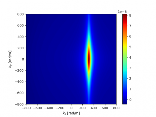
The pressure field induced on a surface by turbulent boundary layer can be an important source of noise and vibration.
Category: CAA
Industrial Applications of CAA
メーカーの技報などネットで公開されている産業界の流体騒音解析に関する資料(日本語)のまとめです.逐次更新していきます.
- 日立アプライアンス
空調機用ファンの大規模数値流体計算
空調機用の遠心ファンの空力騒音の数値計算による予測手法の開発と空力騒音発生メカニズムの解明を目的として,LESによる空力騒音の計算について検討を行っている.ファンの空力騒音は,乱流騒音と翼の回転に起因する回転騒音とに大別できるが,流れ場から発生する乱流騒音が支配的である遠心ファンの場合には,乱流境界層における流れの変動を正確にとらえることが計算精度向上のために必要である.
スーパーコンピュータ「京」を使用して,二種類の遠心ファン形状に対し,およそ6000万と5億要素という計算格子数が異なる二種類のメッシュでそれぞれ計算を行っている.空間解像度が高い5億メッシュの計算の方が,音圧レベル(Sound Pressure Level)や流速分布が実測値に近い結果が得られている.5億メッシュの計算では,どちらの形状についても,1kHz以下の周波数では実験結果と同等の音圧レベルが得られている.更なる計算精度向上を目指して,40億メッシュ規模での計算実行と検証を課題に上げている.
計算の詳細については,論文を参考にとのこと.
- 川崎重工業株式会社
高速鉄道車両の空力騒音解析及びトンネル内すれ違い解析
川崎重工業が開発している CFD 解析ソフト Cflow を使用して,①パンタグラフの空力騒音と②トンネル微気圧波の解析を行っている.①の計算では,遠方観測点における音圧レベルを Curle の式より評価し,風洞試験結果と比較している.
- キヤノン株式会社
電子機器ファンダクト系の空力騒音の数値解析
レイノルズ数 Re が,\(10^4\) ~ \(10^5\) 程度の小型の軸流ファンの空力騒音の直接解析の実現に向けて,FrontFlow/blue を使用して,Dynamic Smagorinsky モデルによる非圧縮 LES 解析を実施している.ファン近傍の領域は回転系として扱い,静止系である上下流領域との情報の交換にオーバーセット法を使用している.この文献内では,空力騒音解析までは実施していない.
- 三菱重工業株式会社
プロペラ翼後流非定常渦の実用的 CFD 解析法の研究
プロペラ翼後縁部から放出されるカルマン渦の発生周波数と翼の固有振動数の一致による共振現象である鳴音(めいおん)の発生予測精度を向上させるための研究.ANSYS Fluent に実装されている RANS モデルと LES モデルのハイブリッド乱流モデルの一種である Embedded LES (ELES) モデルを使用し,領域分割を工夫することにより,設計に適用可能な計算コストで翼の後流に発生する渦を高精度に計算できることを示している.
- 富士電機株式会社
- 株式会社ケーヒン
- 宇宙航空研究開発機構
Computational Aeroacoustics (CAA)

Gallery
- Aeolian Tone (Click the image to start animation 🙂 )

Post Series
- Part1
- Part2
- Part3
- Blade-Vortex Interaction (BVI) Noise
generated by pressure fluctuations near the blade leading edges due to their interactions with the previously generated tip vortices
Open-Source Software for Acoustics Simulation
Coming soon.
Non-reflecting Boundary Conditions in OpenFOAM
- advective & waveTransmissive
- acousticDampingSource
Utilities in OpenFOAM
- probes (Function Objects)
- noise
Case Research
- [Japanese page] Industrial Applications of CAA
Computational Aeroacoustics (CAA) part3
I’ve looked for some benchmark problems in the computational aeroacoustics (CAA) and found the eight problem categories that the BANC (Benchmark Problems for Airframe Noise Computations) workshop has addressed. This workshop is sponsored by the Aeroacoustics Technical Committee.
- Inline Tandem Cylinders
- Minimal 4-wheel Landing Gear (Rudimentary Landing Gear)
- Partially-Dressed Cavity-Closed Nose Landing Gear (PDCC-NLG)
- NASA Slat Noise Configuration (30P30N)
We can access the documents that describe the problem statement by clicking on the link at the bottom of each page:
I’ll try some problems using iconCFD and introduce my results.
| Related Links |
Computational Aeroacoustics (CAA) part2
This is the second in a series of posts about the computational aeroacoustics and I will try to introduce the very basics of the acoustic wave with some pictures.
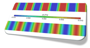
We consider an oscillatory motion with small amplitude in a compressible fluid as shown in the following picture. It shows the distribution of the sound pressure (acoustic pressure) that is defined as the local pressure deviation from the equilibrium pressure \(p_0\) caused by the sound wave propagating from left to right direction.
Since we now consider small oscillations, we can write the local pressure \(p\) and density \(\rho\) in the form
\begin{align}
p &= p_0 + p^{´}, \tag{1a} \label{eq:pressure} \\
\rho &= \rho_0 + \rho^{´}, \tag{1b} \label{eq:density}
\end{align}
where \(p_0\) and \(\rho_0\) are the constant equilibrium pressure and density and \(p^{´}\) and \(\rho^{´}\) are their variations in the sound wave (\(p^{´} \ll p_0, \rho^{´} \ll \rho_0\)), so the above figure is the contour of \(p^{´}\).
We hereafter ignore the fluid viscosity so that only the effect of compressibility is taken into account. Then, the governing equations of the fluid flow is the continuity equation
\begin{align}
\frac{\partial \rho}{\partial t} + \nabla \cdot (\rho \boldsymbol{u}) = 0 \tag{2} \label{eq:continuity}
\end{align}
and the Euler’s equation
\begin{align}
\frac{\partial \boldsymbol{u}}{\partial t} + (\boldsymbol{u} \cdot \nabla)\boldsymbol{u} + \frac{1}{\rho}\nabla p = 0 \tag{3} \label{eq:euler}
\end{align}
where \(\boldsymbol{u}\) is the velocity field. Substituting the eqns. \eqref{eq:pressure} and \eqref{eq:density} into the governing equations and neglecting small quantities of the second order, we get
\begin{align}
\frac{\partial \rho^{´}}{\partial t} + \rho_0 \nabla \cdot \boldsymbol{u} = 0, \tag{4} \label{eq:continuity2}
\end{align}
and
\begin{align}
\frac{\partial \boldsymbol{u}}{\partial t} + \frac{1}{\rho_0} \nabla p^{´} = 0. \tag{5} \label{eq:euler2}
\end{align}
We notice that a sound wave in an ideal fluid is adiabatic and the following relationship holds between the small changes in the pressure and density
\begin{align}
p^{´} = \left(\frac{\partial p}{\partial \rho} \right)_s \rho^{´} \tag{6} \label{eq:adiabatic}
\end{align}
where the subscript s denotes that the partial derivative is taken at constant entropy. Substituting it into \eqref{eq:continuity2}, we get
\begin{align}
\frac{\partial p^{´}}{\partial t} + \rho_0 \left(\frac{\partial p}{\partial \rho} \right)_s \nabla \cdot \boldsymbol{u} = 0. \tag{7} \label{eq:continuity3}
\end{align}
If we introduce the velocity potential \(\boldsymbol{u} = \nabla \phi\), we can derive the relationship between \(p^{´}\) and the potential \(\phi\) from \eqref{eq:euler2}
\begin{align}
p^{´} = -\rho_0 \frac{\partial \phi}{\partial t}. \tag{8} \label{eq:pandphi}
\end{align}
We then obtain the following wave equation from \eqref{eq:continuity3}
\begin{align}
\frac{\partial^2 \phi}{\partial t^2} – c^2 \Delta \phi = 0 \tag{9} \label{eq:waveEqn}
\end{align}
where \(c\) is the speed of sound in an ideal fluid
\begin{align}
c = \sqrt{\left(\frac{\partial p}{\partial \rho} \right)_s}. \tag{10} \label{eq:soundSpeed}
\end{align}
Applying the gradient operator to \eqref{eq:waveEqn}, we find that the each of the three components of the velocity \(\boldsymbol{u}\) satisfies an equation having the same form, and on differentiating \eqref{eq:waveEqn} with respect to time we see that the pressure \(p^{´}\) (and therefore \(\rho^{´}\)) also satisfies the wave equation.
– Landau and Lifshitz, Fluid Mechanics
In a travelling plane wave,
we find
\begin{align}
u_x = \frac{p^{´}}{\rho_0 c}. \tag{11} \label{eq:uxandp}
\end{align}Substituting here from \eqref{eq:adiabatic} \(p^{´} = c^2 \rho^{´}\), we find the relation between the velocity and the density variation:
\begin{align}
u_x = \frac{c \rho^{´}}{\rho_0}. \tag{12} \label{eq:uxandrho}
\end{align}– Landau and Lifshitz, Fluid Mechanics
This book is freely accessible from the link.
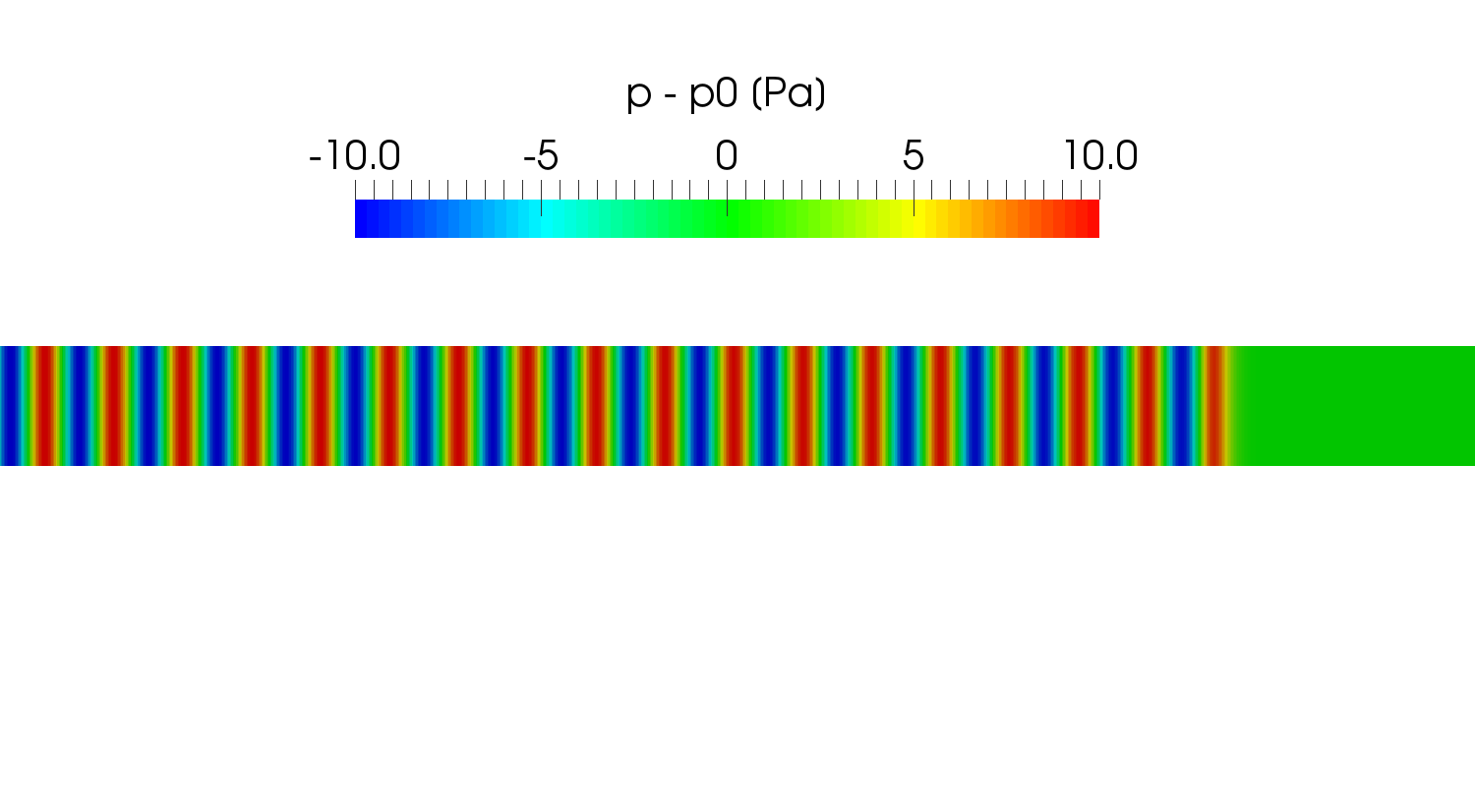
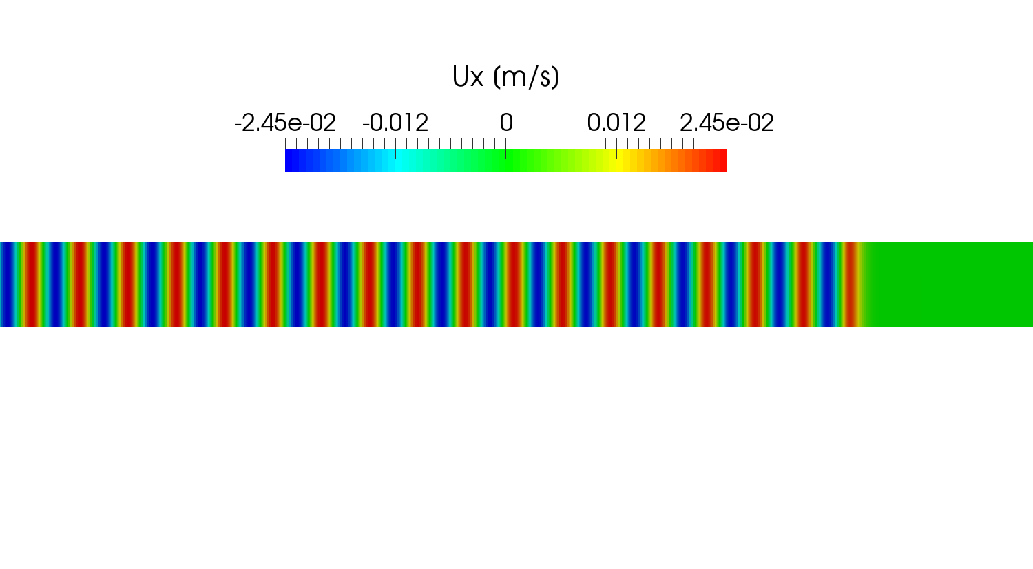
The following picture shows the velocity distribution \(u_x\) calculated using a compressible solver in OpenFOAM at the time corresponding to the pressure variation shown in the above picture. We can calculate the velocity using \eqref{eq:uxandp}
\begin{align}
u_x = \frac{10}{1.2 \times 340} = 0.0245 [m/s]
\end{align}
and it is in good agreement with the result obtained using OpenFOAM.
Computational Aeroacoustics (CAA) part1
This is the first in a series of posts about the computational aeroacoustics that is abbreviated as CAA. Aeroacoustics is mainly concerned with the generation of sound or noise through a fluid flow. Familiar examples are
- Aeolian tone
- Edge tone
- Cavity tone.
They can be studied by both experimental and computational methods. In an experimental approach, the aerodynamically generated sound is measured in the anechoic chamber that is designed to prevent reflections of sound on the wall, making the room echo-free. The following video created by Microsoft will help us to understand the structure of it.
The computational techniques for simulating flow-generated noise can be classified into two broad categories:
| Direct Approaches |
The governing equations of the compressible fluid flow is the compressible Navier-Stokes equations and they also describe the generation and propagation of acoustic noise, so we can solve the computational aeroacoustics problems by solving the transient compressible Navier-Stokes equations both in the source region where the flow disturbances generate noise and propagation region where the generated acoustic waves propagate. Acoustic waves have to be resolved in both regions so that the noise can be accurately simulated at observation locations. However, the solution of the Navier–Stokes equations with fine mesh over large domains to determine farfield noise is computationally very expensive.
As is the case in the experimental approaches, it is essential to prevent the reflection of the acoustic waves on the artificially truncated boundary (i.e. it does not stretch to infinity) of the computational domain in order to obtain an accurate result. A variety of numerical techniques have been developed for this purpose:
- Navier-Stokes Characteristic Boundary Conditions (NSCBC)
- Artificial dissipation and damping in an absorbing zone
- Grid stretching and numerical filtering in a “sponge layer” or “exit zone”
- Perfectly matched layer (PML)
In OpenFOAM, acousticDampingSource is categorized into Ⅱ and the waveTransmissive boundary condition is an approximation of NSCBC.
| Hybrid Approaches (Acoustic Analogy) |
David P. Lockard and Jay H. Casper [1] states that:
The physics-based, airframe noise prediction methodology under investigation is a hybrid of aeroacoustic theory and
computational fluid dynamics (CFD). The near-field aerodynamics associated with an airframe component are simulated to obtain the source input to an acoustic analogy that propagates sound to the far field. The acoustic analogy employed within this current framework is that of Ffowcs Williams and Hawkings, who extended the analogies of Lighthill and Curle to the formulation of aerodynamic sound generated by a surface in arbitrary motion.
- Lighthill’s analogy
Lighthill derived the following wave equation \eqref{eq:Lighthill} from the compressible Navier-Stokes equations:
\begin{align}
\frac{\partial^2 \rho}{\partial t^2} – c_0^2 \nabla^2 \rho = \frac{\partial^2 T_{ij}}{\partial x_i \partial x_j}, \tag{1} \label{eq:Lighthill}
\end{align}
where the so-called Lighthill (turbulence) stress tensor is expressed as
\begin{align}
T_{ij} = \rho u_i u_j + \left( p-c_0^2 \rho \right)\delta_{ij} -\mu \left(\frac{\partial u_i}{\partial x_j} + \frac{\partial u_j}{\partial x_i} – \frac{2}{3}\delta_{ij}\frac{u_k}{x_k} \right), \tag{2} \label{eq:Tij}
\end{align}
\(\delta_{ij}\) is the Kronecker delta and \(c_0\) is the speed of sound in the medium in its equilibrium state.
- Curle’s analogy
The existence of the objects (solid walls) is not considered in the Lighthill’s theory and Curle developed the theory so that it can be dealt with. The density variation at the observer location \(\boldsymbol{x}\) is calculated from the following equation \eqref{eq:Curle}
\begin{align}
\acute{\rho}(\boldsymbol{x}, t) &= \rho(\boldsymbol{x}, t)\;- \rho_0 \\
&=\frac{1}{4 \pi c_0^2} \frac{\partial^2}{\partial x_i \partial x_j} \int_{V}\frac{[T_{ij}]}{r}dV – \frac{1}{4 \pi c_0^2} \frac{\partial}{\partial x_i}\int_{S}\frac{[P_i]}{r}dS, \tag{3} \label{eq:Curle}
\end{align}
where
\begin{align}
P_i = -n_j \{ \delta_{ij}p -\mu \left(\frac{\partial u_i}{\partial x_j} + \frac{\partial u_j}{\partial x_i} – \frac{2}{3}\delta_{ij}\frac{u_k}{x_k} \right) \}, \tag{4} \label{eq:Pi}
\end{align}
\(r\) is the distance between the receiver \(\boldsymbol{x}\) and the source position \(\boldsymbol{y}\) in \(V\) (or on \(S\)) and the operator [] denotes evaluation at the retarded time \(t-r/c_0\).
- Ffowcs-Williams and Hawkings (FW-H) analogy
In the following video, we can watch the lecture by James Lighthill and John Ffowcs Williams !
| References (English) |
- [1] Permeable Surface Corrections for Ffowcs Williams and Hawkings Integrals
- [2] CFD Online – Acoustic Solver with openfoam
- [3] WIKIBOOKS – Engineering Acoustics/Analogies in aeroacoustics
| References (Japanese) |
- [4] 加藤千幸,大規模数値流体解析による流体音の予測
- [5] 飯田明由,送風機(ファン)の騒音発生メカニズムと低減・静粛化対策とその事例
- [6] 大嶋拓也,流れ中の柱状物体列から発生する空力音の数値予測に関する研究
- [7] Newsletters Nagare Dec. issue 2010