Description
Apply a simplified boundary-layer model to the velocity and turbulence fields based on the 1/7th power-law.
The uniform boundary-layer thickness is either provided via the -ybl option or calculated as the average of the distance to the wall scaled with the thickness coefficient supplied via the option -Cbl. If both options are provided -ybl is used.
The velocity profile is initialized based on the 1/7th power law turbulent velocity profile:
\begin{equation}
\boldsymbol{u} = \boldsymbol{U} \left( \frac{y_w}{\delta} \right)^{\frac{1}{7}}, \tag{1}
\end{equation}
where \(\boldsymbol{U}\) is the main flow velocity, \(y_w\) is the distance to the wall and \(\delta\) is the boundary-layer thickness.
applyBoundaryLayer.C
C++
101
102
103
104
105
106
107
108
109
110
111
112
113
114
115
116
117
118
119
120
121
122
// Modify velocity by applying a 1/7th power law boundary-layer
// u/U0 = (y/ybl)^(1/7)
// assumes U0 is the same as the current cell velocity
When we discretize the partial differential equations using the Finite Volume Method (FVM), we get sets of linear algebraic equations with large sparse coefficient matrices that are solved using iterative or direct methods. There is renumberMesh utility in OpenFOAM that is used to reduce the bandwidth of the coefficient matrices by renumbering the cell label list.
The bandwidth is not a special term in OpenFOAM but it is a general concept in the field of solving linear systems of equations. In this blog post, I will try to give a description of it and other important terms such as profile and frontwidth.
The definitions of these terms are clearly described in [1]. Let \(A\) be an \(N\) by \(N\) matrix with symmetric zero-nonzero structure, i.e. , \(a_{ij} \neq 0\) if and only if \(a_{ji} \neq 0\).
When the renumberMesh utility is executed, the following data is reported to the screen.
Log of renumberMesh
Shell
1
2
3
4
5
6
7
8
9
10
11
12
13
14
15
16
17
18
19
20
21
22
23
24
25
26
27
28
Create time
Create mesh fortime=0
Mesh size:245760
Before renumbering:
band:217487
profile:2793999079
rms frontwidth:12694.49013
Renumber according torenumberMeshDict
Writing renumber maps(newtoold)topolyMesh.
Selecting renumberMethod CuthillMcKee
After renumbering:
band:978
profile:226514746
rms frontwidth:932.0721888
Writing mesh to"1"
Written current cellID andorigCellID asvolScalarField foruseinpostprocessing.
End
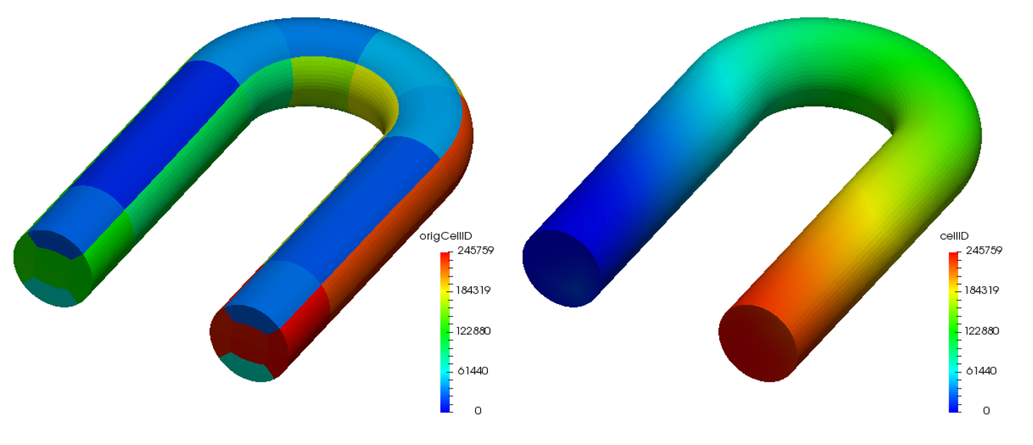
Here, the band, profile and rms frontwidth correspond to \eqref{eq:Bandwidth}, \eqref{eq:Profile} and \eqref{eq:rmsFrontwidth}, respectively. We can confirm that they all decreased after renumbering the cell label using the Cuthill-McKee (CM) algorithm. The distributions of cell labels are visually compared between before and after reordering operations in Figure 1.
Fig. 1 (Left) Before reordering, (Right) After reordering.
Source code of renumberMesh utility
getBand function | renumberMesh.C
C++
116
117
118
119
120
121
122
123
124
125
126
127
128
129
130
131
132
133
134
135
136
137
138
139
140
141
142
143
144
145
146
147
148
149
150
151
152
153
154
155
156
157
158
159
160
161
162
163
// Calculate band of matrix
voidgetBand
(
constboolcalculateIntersect,
constlabel nCells,
constlabelList&owner,
constlabelList&neighbour,
label&bandwidth,
scalar&profile,// scalar to avoid overflow
scalar&sumSqrIntersect// scalar to avoid overflow
)
{
labelList cellBandwidth(nCells,0);
scalarField nIntersect(nCells,0.0);
forAll(neighbour,facei)
{
label own=owner[facei];
label nei=neighbour[facei];
// Note: mag not necessary for correct (upper-triangular) ordering.
label diff=nei-own;
cellBandwidth[nei]=max(cellBandwidth[nei],diff);
}
bandwidth=max(cellBandwidth);
// Do not use field algebra because of conversion label to scalar
The getBand function is called from the main function. The variables band, profile and rmsFrontwidth represent \eqref{eq:Bandwidth}, \eqref{eq:Profile} and \eqref{eq:rmsFrontwidth}, respectively.
After the simulation has finished, you can do simple calculation, such as addition and subtraction, with the field data using foamCalc utility. The source code is located in the following directories:
applications/utilities/postProcessing/foamCalc
src/postProcessing/foamCalcFunctions.
components
$ foamCalc components U -latestTime
This example is to generate three component files Ux, Uy and Uz (volScalarField) from volVectorFieldU only at the latest time directory.
mag
$ foamCalc mag U
This example is to generate velocity magnitude field \(|\boldsymbol{U}|\) file magU at every existing time directory.
magSqr
$ foamCalc magSqr U
This example is to generate magnitude squared field \(|\boldsymbol{U}|^2\) file magSqrU at every existing time directory.
This example is to convert the temperature unit from Kelvin to degrees at time 5000. The generated file name can be specified using –resultName option.
div
$ foamCalc div phi
This example is to calculate the divergence of the flux field phi for the estimation of the continuity error of each cell for incompressible flow.
interpolate
$ foamCalc interpolate T -latestTime
This example it to generate surfaceScalarFieldinterpolateT from volScalarFieldT using the interpolation scheme specified in the system/fvSchemes file.