# The data in this file was extracted from a direct numerical
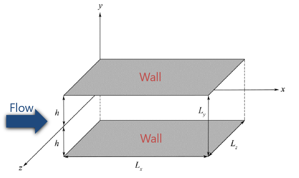
# simulation of fully developed plane turbulent channel
# flow. Particulars are listed below. Note that some of the statistical
# quantities provided in this data set should be zero due to
# (statistical) symmetries in the flow. These quantities are reported
# here none-the-less as an indicator of the quality of the statistics.
# more statistics from this data set are available at
# http://www.tam.uiuc.edu/Faculty/Moser/channel
#
# Authors: Moser, Kim & Mansour
# Reference: DNS of Turbulent Channel Flow up to Re_tau=590, 1999,
# Physics of Fluids, vol 11, 943-945.
# Numerical Method: Kim, Moin & Moser, 1987, J. Fluid Mech. vol 177, 133-166
# Re_tau = 392.24
# Normalization: U_tau, h
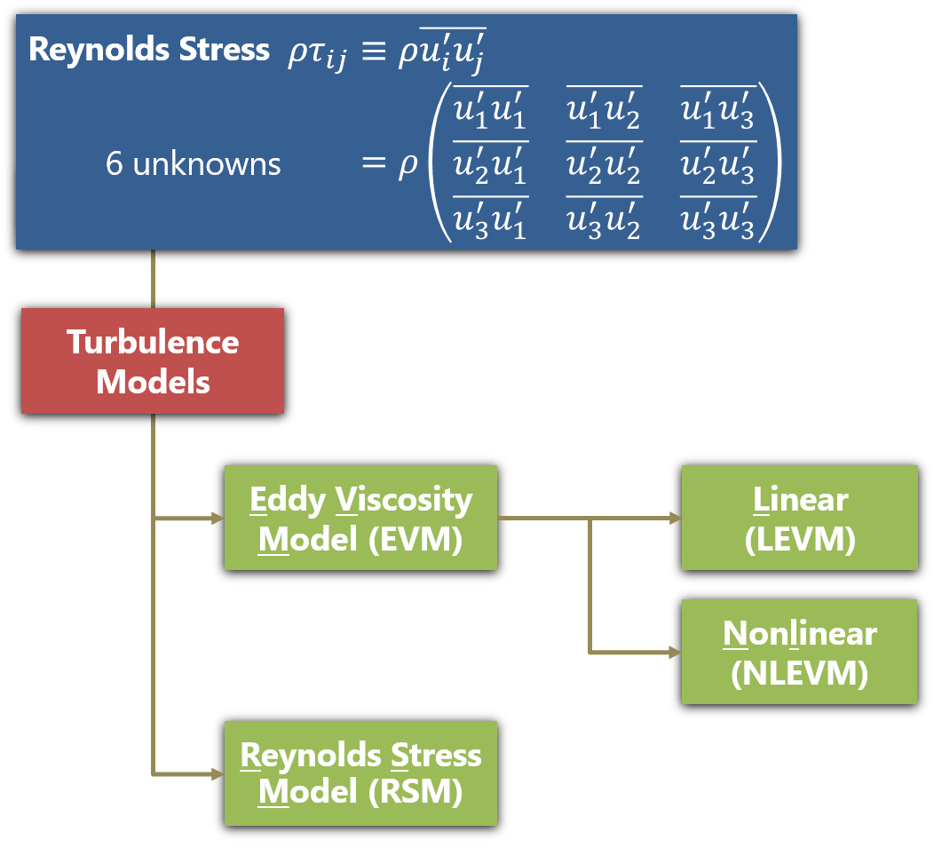
# Description: Components of the Reynolds stress tensor
# Filename: chan395/profiles/chan395.reystress
# Date File Created: Mar 01, 2000
#
#---End of Header---
#
# ny = 257, Re = 392.24
#
# y y+ R_uu R_vv R_ww R_uv R_uw R_vw
#
0.0000e+00 0.0000e+00 5.3376e-28 4.9018e-29 5.9575e-28 1.1206e-30 -6.1282e-30 6.2793e-32
7.5298e-05 2.9535e-02 1.3684e-04 9.4734e-11 5.2943e-05 -2.4414e-08 5.9464e-08 -2.8525e-11
3.0118e-04 1.1814e-01 2.1828e-03 2.3603e-08 8.2715e-04 -1.5728e-06 8.3228e-07 -1.7141e-09
6.7762e-04 2.6579e-01 1.1020e-02 5.7878e-07 4.0392e-03 -1.8113e-05 3.3616e-06 -1.9051e-08
1.2045e-03 4.7248e-01 3.4718e-02 5.4400e-06 1.2147e-02 -1.0324e-04 1.0732e-05 -1.0411e-07
1.8819e-03 7.3816e-01 8.4454e-02 3.0014e-05 2.7852e-02 -4.0027e-04 2.8297e-05 -3.8272e-07
2.7095e-03 1.0628e+00 1.7438e-01 1.1756e-04 5.3564e-02 -1.2143e-03 6.6865e-05 -1.0969e-06
3.6874e-03 1.4464e+00 3.2123e-01 3.6204e-04 9.0947e-02 -3.1009e-03 1.4506e-04 -2.6288e-06
4.8153e-03 1.8888e+00 5.4336e-01 9.3203e-04 1.4062e-01 -6.9486e-03 2.9097e-04 -5.4596e-06
6.0930e-03 2.3900e+00 8.5851e-01 2.0879e-03 2.0209e-01 -1.4015e-02 5.4723e-04 -1.0091e-05
7.5205e-03 2.9499e+00 1.2802e+00 4.1852e-03 2.7384e-01 -2.5858e-02 9.7373e-04 -1.7119e-05
9.0974e-03 3.5684e+00 1.8132e+00 7.6610e-03 3.5369e-01 -4.4135e-02 1.6529e-03 -2.7764e-05
1.0823e-02 4.2455e+00 2.4490e+00 1.3005e-02 4.3919e-01 -7.0276e-02 2.6847e-03 -4.4587e-05
1.2699e-02 4.9810e+00 3.1644e+00 2.0724e-02 5.2804e-01 -1.0513e-01 4.1721e-03 -7.1044e-05
1.4722e-02 5.7748e+00 3.9229e+00 3.1300e-02 6.1834e-01 -1.4869e-01 6.1889e-03 -1.0893e-04
1.6895e-02 6.6268e+00 4.6811e+00 4.5157e-02 7.0871e-01 -1.9999e-01 8.7562e-03 -1.5460e-04
1.9215e-02 7.5369e+00 5.3953e+00 6.2636e-02 7.9819e-01 -2.5724e-01 1.1834e-02 -1.9552e-04
2.1683e-02 8.5049e+00 6.0286e+00 8.3971e-02 8.8610e-01 -3.1808e-01 1.5387e-02 -2.1029e-04
2.4298e-02 9.5307e+00 6.5558e+00 1.0928e-01 9.7178e-01 -3.8001e-01 1.9449e-02 -1.7262e-04
2.7060e-02 1.0614e+01 6.9642e+00 1.3854e-01 1.0545e+00 -4.4073e-01 2.4133e-02 -6.0490e-05
2.9969e-02 1.1755e+01 7.2524e+00 1.7162e-01 1.1333e+00 -4.9837e-01 2.9501e-02 1.3268e-04
3.3024e-02 1.2953e+01 7.4274e+00 2.0824e-01 1.2075e+00 -5.5162e-01 3.5418e-02 3.9086e-04
3.6224e-02 1.4209e+01 7.5016e+00 2.4803e-01 1.2762e+00 -5.9969e-01 4.1511e-02 6.7818e-04
3.9569e-02 1.5521e+01 7.4897e+00 2.9050e-01 1.3387e+00 -6.4224e-01 4.7330e-02 9.5511e-04
4.3060e-02 1.6890e+01 7.4069e+00 3.3510e-01 1.3948e+00 -6.7924e-01 5.2512e-02 1.1989e-03
4.6694e-02 1.8315e+01 7.2679e+00 3.8121e-01 1.4444e+00 -7.1090e-01 5.6926e-02 1.4016e-03
5.0472e-02 1.9797e+01 7.0865e+00 4.2818e-01 1.4878e+00 -7.3759e-01 6.0659e-02 1.5532e-03
5.4393e-02 2.1335e+01 6.8750e+00 4.7535e-01 1.5251e+00 -7.5980e-01 6.3835e-02 1.6360e-03
5.8456e-02 2.2929e+01 6.6441e+00 5.2211e-01 1.5568e+00 -7.7810e-01 6.6418e-02 1.6465e-03
6.2661e-02 2.4578e+01 6.4025e+00 5.6790e-01 1.5833e+00 -7.9302e-01 6.8207e-02 1.6026e-03
6.7007e-02 2.6283e+01 6.1573e+00 6.1229e-01 1.6047e+00 -8.0503e-01 6.9001e-02 1.5073e-03
7.1494e-02 2.8043e+01 5.9141e+00 6.5493e-01 1.6216e+00 -8.1452e-01 6.8896e-02 1.3268e-03
7.6120e-02 2.9858e+01 5.6767e+00 6.9554e-01 1.6344e+00 -8.2184e-01 6.8285e-02 1.0303e-03
8.0886e-02 3.1727e+01 5.4477e+00 7.3388e-01 1.6439e+00 -8.2733e-01 6.7481e-02 6.4119e-04
8.5790e-02 3.3651e+01 5.2291e+00 7.6971e-01 1.6512e+00 -8.3133e-01 6.6450e-02 2.3642e-04
9.0832e-02 3.5628e+01 5.0223e+00 8.0285e-01 1.6567e+00 -8.3412e-01 6.4937e-02 -1.3612e-04
9.6011e-02 3.7660e+01 4.8279e+00 8.3316e-01 1.6606e+00 -8.3590e-01 6.2875e-02 -4.7569e-04
1.0133e-01 3.9744e+01 4.6462e+00 8.6061e-01 1.6623e+00 -8.3683e-01 6.0710e-02 -7.8412e-04
1.0678e-01 4.1882e+01 4.4768e+00 8.8520e-01 1.6618e+00 -8.3700e-01 5.9182e-02 -1.0539e-03
1.1236e-01 4.4073e+01 4.3194e+00 9.0700e-01 1.6594e+00 -8.3649e-01 5.8527e-02 -1.2655e-03
1.1808e-01 4.6316e+01 4.1730e+00 9.2607e-01 1.6553e+00 -8.3523e-01 5.8437e-02 -1.4126e-03
1.2393e-01 4.8611e+01 4.0370e+00 9.4247e-01 1.6500e+00 -8.3321e-01 5.8512e-02 -1.4930e-03
1.2991e-01 5.0958e+01 3.9106e+00 9.5626e-01 1.6439e+00 -8.3044e-01 5.8376e-02 -1.5118e-03
1.3603e-01 5.3356e+01 3.7930e+00 9.6754e-01 1.6373e+00 -8.2687e-01 5.8084e-02 -1.5196e-03
1.4227e-01 5.5805e+01 3.6834e+00 9.7651e-01 1.6299e+00 -8.2252e-01 5.8125e-02 -1.6228e-03
1.4864e-01 5.8305e+01 3.5821e+00 9.8341e-01 1.6209e+00 -8.1762e-01 5.8537e-02 -1.8295e-03
1.5515e-01 6.0855e+01 3.4896e+00 9.8850e-01 1.6105e+00 -8.1249e-01 5.8809e-02 -2.0145e-03
1.6178e-01 6.3456e+01 3.4053e+00 9.9197e-01 1.5991e+00 -8.0726e-01 5.8494e-02 -2.0826e-03
1.6853e-01 6.6105e+01 3.3278e+00 9.9396e-01 1.5872e+00 -8.0180e-01 5.7876e-02 -2.1101e-03
1.7541e-01 6.8804e+01 3.2557e+00 9.9455e-01 1.5754e+00 -7.9592e-01 5.7034e-02 -2.1628e-03
1.8242e-01 7.1551e+01 3.1886e+00 9.9379e-01 1.5637e+00 -7.8961e-01 5.5746e-02 -2.2441e-03
1.8954e-01 7.4347e+01 3.1269e+00 9.9183e-01 1.5510e+00 -7.8296e-01 5.4259e-02 -2.3220e-03
1.9679e-01 7.7191e+01 3.0702e+00 9.8887e-01 1.5367e+00 -7.7613e-01 5.2957e-02 -2.3519e-03
2.0416e-01 8.0082e+01 3.0178e+00 9.8512e-01 1.5212e+00 -7.6929e-01 5.1819e-02 -2.3018e-03
2.1165e-01 8.3020e+01 2.9678e+00 9.8075e-01 1.5052e+00 -7.6243e-01 5.0872e-02 -2.0851e-03
2.1926e-01 8.6005e+01 2.9191e+00 9.7583e-01 1.4889e+00 -7.5552e-01 5.0514e-02 -1.6209e-03
2.2699e-01 8.9035e+01 2.8712e+00 9.7044e-01 1.4721e+00 -7.4851e-01 5.0564e-02 -8.5802e-04
2.3483e-01 9.2112e+01 2.8239e+00 9.6465e-01 1.4551e+00 -7.4146e-01 5.0229e-02 1.1783e-04
2.4279e-01 9.5234e+01 2.7776e+00 9.5846e-01 1.4379e+00 -7.3445e-01 4.9171e-02 1.0337e-03
2.5086e-01 9.8400e+01 2.7324e+00 9.5179e-01 1.4206e+00 -7.2737e-01 4.7565e-02 1.6440e-03
2.5905e-01 1.0161e+02 2.6883e+00 9.4459e-01 1.4035e+00 -7.2012e-01 4.5716e-02 1.9851e-03
2.6735e-01 1.0486e+02 2.6453e+00 9.3679e-01 1.3867e+00 -7.1271e-01 4.3916e-02 2.2291e-03
2.7575e-01 1.0816e+02 2.6031e+00 9.2845e-01 1.3696e+00 -7.0521e-01 4.2134e-02 2.4143e-03
2.8427e-01 1.1150e+02 2.5612e+00 9.1976e-01 1.3515e+00 -6.9761e-01 4.0077e-02 2.5128e-03
2.9289e-01 1.1489e+02 2.5196e+00 9.1087e-01 1.3322e+00 -6.8985e-01 3.7520e-02 2.5006e-03
3.0162e-01 1.1831e+02 2.4793e+00 9.0185e-01 1.3118e+00 -6.8192e-01 3.4358e-02 2.3726e-03
3.1046e-01 1.2178e+02 2.4411e+00 8.9268e-01 1.2910e+00 -6.7396e-01 3.0858e-02 2.1952e-03
3.1940e-01 1.2528e+02 2.4055e+00 8.8335e-01 1.2700e+00 -6.6598e-01 2.7094e-02 2.0517e-03
3.2844e-01 1.2883e+02 2.3714e+00 8.7385e-01 1.2488e+00 -6.5794e-01 2.3371e-02 1.9999e-03
3.3758e-01 1.3242e+02 2.3380e+00 8.6418e-01 1.2276e+00 -6.4977e-01 2.0500e-02 1.9700e-03
3.4683e-01 1.3604e+02 2.3046e+00 8.5436e-01 1.2066e+00 -6.4148e-01 1.8795e-02 1.8189e-03
3.5617e-01 1.3971e+02 2.2708e+00 8.4439e-01 1.1855e+00 -6.3298e-01 1.7891e-02 1.4336e-03
3.6561e-01 1.4341e+02 2.2365e+00 8.3421e-01 1.1641e+00 -6.2415e-01 1.7572e-02 7.5375e-04
3.7514e-01 1.4715e+02 2.2023e+00 8.2369e-01 1.1423e+00 -6.1500e-01 1.7517e-02 -7.9290e-05
3.8477e-01 1.5092e+02 2.1682e+00 8.1285e-01 1.1202e+00 -6.0551e-01 1.7095e-02 -8.3720e-04
3.9449e-01 1.5474e+02 2.1335e+00 8.0181e-01 1.0983e+00 -5.9561e-01 1.5913e-02 -1.3413e-03
4.0430e-01 1.5858e+02 2.0983e+00 7.9074e-01 1.0767e+00 -5.8530e-01 1.4306e-02 -1.5771e-03
4.1420e-01 1.6247e+02 2.0631e+00 7.7968e-01 1.0551e+00 -5.7460e-01 1.2812e-02 -1.5179e-03
4.2419e-01 1.6639e+02 2.0277e+00 7.6856e-01 1.0339e+00 -5.6350e-01 1.1907e-02 -1.1762e-03
4.3427e-01 1.7034e+02 1.9920e+00 7.5731e-01 1.0131e+00 -5.5204e-01 1.1640e-02 -7.0498e-04
4.4443e-01 1.7433e+02 1.9568e+00 7.4588e-01 9.9279e-01 -5.4040e-01 1.1503e-02 -2.0689e-04
4.5467e-01 1.7834e+02 1.9229e+00 7.3425e-01 9.7254e-01 -5.2883e-01 1.1097e-02 2.0529e-04
4.6500e-01 1.8239e+02 1.8896e+00 7.2249e-01 9.5187e-01 -5.1747e-01 1.0218e-02 5.0971e-04
4.7541e-01 1.8648e+02 1.8562e+00 7.1064e-01 9.3057e-01 -5.0626e-01 9.0004e-03 7.6211e-04
4.8590e-01 1.9059e+02 1.8232e+00 6.9862e-01 9.0936e-01 -4.9507e-01 7.8753e-03 9.2292e-04
4.9646e-01 1.9473e+02 1.7908e+00 6.8642e-01 8.8926e-01 -4.8386e-01 7.1617e-03 9.3017e-04
5.0710e-01 1.9891e+02 1.7591e+00 6.7417e-01 8.7042e-01 -4.7269e-01 7.0121e-03 7.2814e-04
5.1782e-01 2.0311e+02 1.7274e+00 6.6201e-01 8.5243e-01 -4.6164e-01 7.3802e-03 2.7352e-04
5.2860e-01 2.0734e+02 1.6948e+00 6.5007e-01 8.3469e-01 -4.5072e-01 8.2299e-03 -2.9303e-04
5.3946e-01 2.1160e+02 1.6610e+00 6.3843e-01 8.1690e-01 -4.3999e-01 9.3954e-03 -7.4565e-04
5.5039e-01 2.1589e+02 1.6264e+00 6.2712e-01 7.9939e-01 -4.2949e-01 1.0585e-02 -9.5384e-04
5.6138e-01 2.2020e+02 1.5910e+00 6.1613e-01 7.8241e-01 -4.1910e-01 1.1834e-02 -9.5389e-04
5.7244e-01 2.2454e+02 1.5550e+00 6.0545e-01 7.6587e-01 -4.0876e-01 1.3728e-02 -1.0075e-03
5.8357e-01 2.2890e+02 1.5184e+00 5.9512e-01 7.4931e-01 -3.9853e-01 1.6563e-02 -1.2970e-03
5.9476e-01 2.3329e+02 1.4808e+00 5.8523e-01 7.3258e-01 -3.8843e-01 1.9835e-02 -1.7620e-03
6.0601e-01 2.3770e+02 1.4425e+00 5.7589e-01 7.1572e-01 -3.7835e-01 2.2555e-02 -2.2305e-03
6.1732e-01 2.4214e+02 1.4037e+00 5.6715e-01 6.9868e-01 -3.6810e-01 2.3965e-02 -2.5637e-03
6.2868e-01 2.4660e+02 1.3647e+00 5.5896e-01 6.8159e-01 -3.5761e-01 2.4099e-02 -2.7183e-03
6.4010e-01 2.5108e+02 1.3260e+00 5.5120e-01 6.6492e-01 -3.4695e-01 2.3378e-02 -2.7095e-03
6.5158e-01 2.5558e+02 1.2881e+00 5.4372e-01 6.4916e-01 -3.3621e-01 2.2236e-02 -2.5722e-03
6.6311e-01 2.6010e+02 1.2513e+00 5.3642e-01 6.3424e-01 -3.2544e-01 2.0871e-02 -2.4646e-03
6.7469e-01 2.6464e+02 1.2162e+00 5.2919e-01 6.2001e-01 -3.1468e-01 1.9224e-02 -2.5472e-03
6.8632e-01 2.6920e+02 1.1827e+00 5.2197e-01 6.0660e-01 -3.0393e-01 1.7273e-02 -2.7871e-03
6.9799e-01 2.7378e+02 1.1500e+00 5.1473e-01 5.9377e-01 -2.9315e-01 1.5116e-02 -3.0094e-03
7.0972e-01 2.7838e+02 1.1175e+00 5.0750e-01 5.8101e-01 -2.8231e-01 1.3055e-02 -3.1202e-03
7.2148e-01 2.8300e+02 1.0843e+00 5.0029e-01 5.6815e-01 -2.7133e-01 1.1360e-02 -3.1772e-03
7.3329e-01 2.8763e+02 1.0507e+00 4.9312e-01 5.5541e-01 -2.6019e-01 9.9787e-03 -3.2410e-03
7.4513e-01 2.9227e+02 1.0173e+00 4.8605e-01 5.4304e-01 -2.4893e-01 8.7677e-03 -3.3171e-03
7.5702e-01 2.9694e+02 9.8478e-01 4.7922e-01 5.3113e-01 -2.3753e-01 7.8868e-03 -3.3738e-03
7.6894e-01 3.0161e+02 9.5377e-01 4.7268e-01 5.1971e-01 -2.2605e-01 7.6156e-03 -3.4135e-03
7.8090e-01 3.0630e+02 9.2454e-01 4.6644e-01 5.0882e-01 -2.1462e-01 7.9424e-03 -3.4897e-03
7.9289e-01 3.1101e+02 8.9706e-01 4.6047e-01 4.9853e-01 -2.0326e-01 8.6379e-03 -3.6720e-03
8.0491e-01 3.1572e+02 8.7113e-01 4.5478e-01 4.8883e-01 -1.9188e-01 9.5840e-03 -3.9882e-03
8.1696e-01 3.2045e+02 8.4645e-01 4.4932e-01 4.7982e-01 -1.8043e-01 1.0540e-02 -4.3896e-03
8.2904e-01 3.2519e+02 8.2296e-01 4.4410e-01 4.7164e-01 -1.6898e-01 1.1159e-02 -4.7685e-03
8.4114e-01 3.2993e+02 8.0062e-01 4.3915e-01 4.6392e-01 -1.5752e-01 1.1209e-02 -5.0417e-03
8.5327e-01 3.3469e+02 7.7929e-01 4.3458e-01 4.5618e-01 -1.4601e-01 1.0617e-02 -5.1687e-03
8.6542e-01 3.3946e+02 7.5889e-01 4.3044e-01 4.4842e-01 -1.3442e-01 9.5260e-03 -5.1040e-03
8.7759e-01 3.4423e+02 7.3932e-01 4.2671e-01 4.4071e-01 -1.2272e-01 8.2998e-03 -4.8287e-03
8.8978e-01 3.4901e+02 7.2051e-01 4.2339e-01 4.3345e-01 -1.1094e-01 7.2287e-03 -4.4056e-03
9.0198e-01 3.5380e+02 7.0261e-01 4.2046e-01 4.2708e-01 -9.9120e-02 6.4502e-03 -3.8984e-03
9.1420e-01 3.5859e+02 6.8576e-01 4.1796e-01 4.2169e-01 -8.7301e-02 6.1696e-03 -3.3462e-03
9.2644e-01 3.6339e+02 6.7023e-01 4.1591e-01 4.1709e-01 -7.5441e-02 6.4277e-03 -2.7927e-03
9.3868e-01 3.6819e+02 6.5620e-01 4.1431e-01 4.1319e-01 -6.3452e-02 7.0238e-03 -2.2376e-03
9.5093e-01 3.7300e+02 6.4389e-01 4.1313e-01 4.0984e-01 -5.1252e-02 7.7818e-03 -1.6855e-03
9.6319e-01 3.7781e+02 6.3375e-01 4.1234e-01 4.0689e-01 -3.8772e-02 8.7489e-03 -1.1858e-03
9.7546e-01 3.8262e+02 6.2626e-01 4.1188e-01 4.0431e-01 -2.6001e-02 9.8627e-03 -7.6554e-04
9.8773e-01 3.8743e+02 6.2174e-01 4.1166e-01 4.0247e-01 -1.3031e-02 1.0731e-02 -3.8835e-04
1.0000e-00 3.9224e+02 6.2024e-01 4.1160e-01 4.0179e-01 0.0000e+00 1.1032e-02 0.0000e+00