The mathematical expressions of the viscous stress differ between Newtonian fluids and non-Newtonian fluids, so do those of the diffusion term. In this post, we consider only Newtonian fluids, such as air and water.
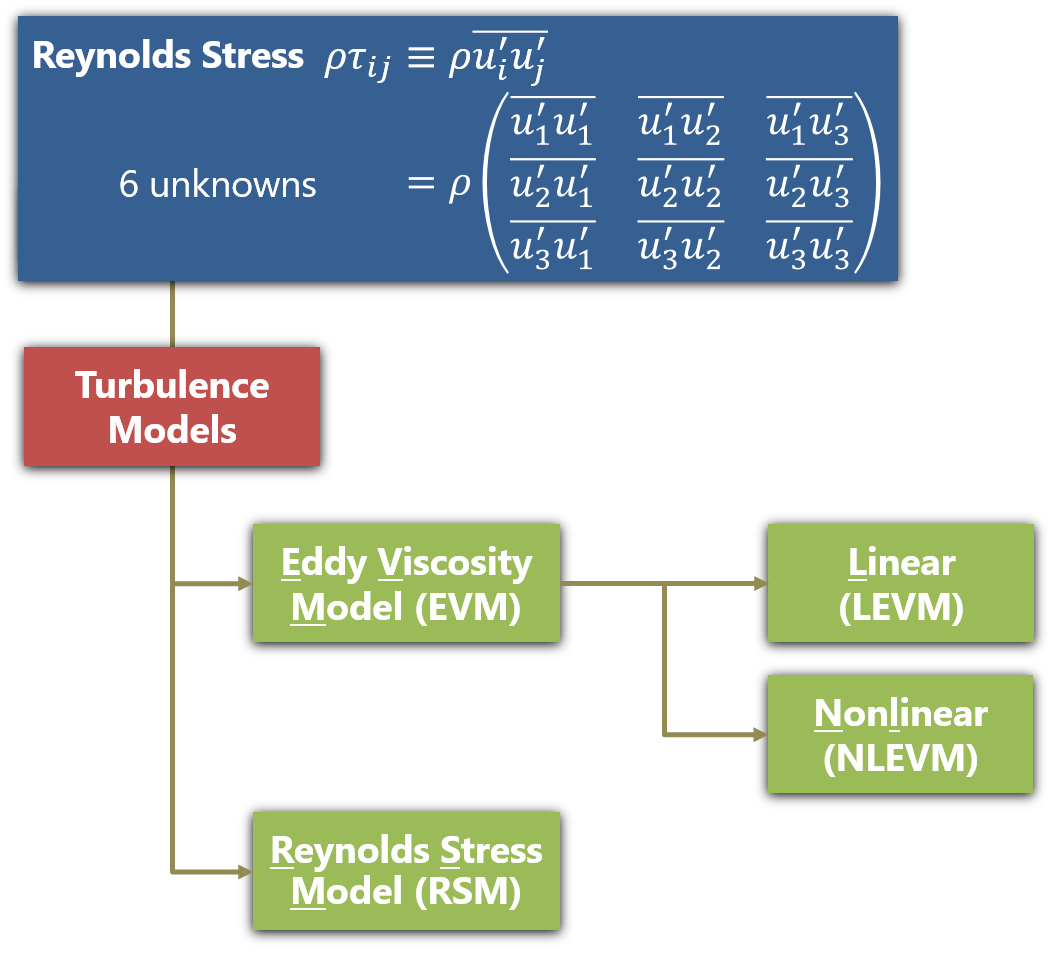
Many turbulence models treat the effects of the turbulence as augmentation of mixing or diffusion, but the modeled expression differs depending on the turbulence models, such as linear eddy-viscosity, non-linear eddy viscosity and Reynolds-stress transport models.
We’ll start by running through mathematical expressions of the diffusion term and find out how these are implemented in OpenFOAM.
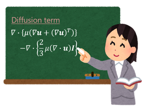
Diffusion term (Newtonian fluids)
For Newtonian fluids the ratio of the shear stress to the shear rate is constant and the diffusion term of the Navier-Stokes equations are given by:
\begin{equation}
\nabla \cdot \left( \mu \left( \nabla \boldsymbol{u} + (\nabla \boldsymbol{u})^T \right) -\frac{2}{3}\mu (\nabla \cdot \boldsymbol{u}) \boldsymbol{I} \right), \tag{1} \label{eq:newtondiffusion}
\end{equation}
where \(\boldsymbol{u}\) is the velocity field, \(\mu\) is the molecular viscosity and \(\boldsymbol{I}\) is the identity tensor.
In the case of laminar flows and Direct Numerical Simulations (DNS) of turbulent flows, this expression is used.
When we solve turbulent flows with turbulence models, the expression of the diffusion term changes from Eq. \eqref{eq:newtondiffusion} according to the model we choose. If we use the linear eddy-viscosity models of Reynolds-averaged Navier-Stokes (RANS), such as k-\(\epsilon\) and k-\(\omega\) SST models, the Reynolds stress is modeled with the following expression:
\begin{equation}
-\rho\overline{\boldsymbol{u}\boldsymbol{u}} = \mu_t \left( \nabla \overline{\boldsymbol{u}} + (\nabla \overline{\boldsymbol{u}})^T \right) -\frac{2}{3}\rho k \boldsymbol{I}, \tag{2} \label{eq:BoussinesqApprox}
\end{equation}
and the diffusion term is expressed as:
\begin{align}
&\nabla \cdot \left( \mu \left( \nabla \overline{\boldsymbol{u}} + (\nabla \overline{\boldsymbol{u}})^T \right) -\frac{2}{3}\mu (\nabla \cdot \overline{\boldsymbol{u}}) \boldsymbol{I} -\rho\overline{\boldsymbol{u}\boldsymbol{u}} \right) \\
=& \nabla \cdot \left( (\mu + \mu_t) \left( \nabla \overline{\boldsymbol{u}} + (\nabla \overline{\boldsymbol{u}})^T \right) -\frac{2}{3}\mu (\nabla \cdot \overline{\boldsymbol{u}}) \boldsymbol{I} – \frac{2}{3}\rho k \boldsymbol{I} \right) \\
=& \nabla \cdot \left( \mu_{eff} \left( \nabla \overline{\boldsymbol{u}} + (\nabla \overline{\boldsymbol{u}})^T \right) -\frac{2}{3}\mu (\nabla \cdot \overline{\boldsymbol{u}}) \boldsymbol{I} \right) – \nabla \cdot \left( \frac{2}{3}\rho k \boldsymbol{I} \right), \tag{3} \label{eq:levmdiffusion}
\end{align}
where \(\overline{\boldsymbol{u}}\) is the ensemble-averaged velocity field, \(k\) is the turbulence energy, \(\rho\) is the density and the effective viscosity \(\mu_{eff}\) is the sum of the molecular and turbulent eddy viscosity \(\mu_t\).
If the flow is incompressible, the expression reduces to the following one because of the continuity equation \(\nabla \cdot \overline{\boldsymbol{u}} = 0\):
\begin{equation}
\nabla \cdot \left( \mu_{eff} \left( \nabla \overline{\boldsymbol{u}} + (\nabla \overline{\boldsymbol{u}})^T \right) \right) – \nabla \cdot \left( \frac{2}{3}\rho k \boldsymbol{I} \right). \tag{4} \label{eq:incompdiffusion}
\end{equation}
If turbulence models of the eddy-viscosity type is used, the effects of fluctuating turbulent flows are expressed as augmentation of the diffusion as can be seen from Eq. \eqref{eq:levmdiffusion}.
We are all set!
Let’s look into how the diffusion term is handled in OpenFOAM 🙂
Implementation in OpenFOAM
If we have a quick look at UEqn.H file of rhoPimpleFoam, a transient compressible flow solver, we can find turbulence->divDevRhoReff(U) in it. It corresponds to the diffusion term.
|
1 2 3 4 5 6 7 8 9 10 11 12 13 14 15 16 17 18 19 20 21 22 23 24 25 |
// Solve the Momentum equation MRF.correctBoundaryVelocity(U); tmp<fvVectorMatrix> tUEqn ( fvm::ddt(rho, U) + fvm::div(phi, U) + MRF.DDt(rho, U) + turbulence->divDevRhoReff(U) == fvOptions(rho, U) ); fvVectorMatrix& UEqn = tUEqn.ref(); UEqn.relax(); fvOptions.constrain(UEqn); if (pimple.momentumPredictor()) { solve(UEqn == -fvc::grad(p)); fvOptions.correct(U); K = 0.5*magSqr(U); } |
We can find its definitions in different files depending on the types of the turbulence models. In the case of linear eddy viscosity models, it is defined in linearViscousStress.C file.
|
1 2 3 4 5 6 7 8 9 10 11 12 13 |
template<class BasicTurbulenceModel> Foam::tmp<Foam::fvVectorMatrix> Foam::linearViscousStress<BasicTurbulenceModel>::divDevRhoReff ( volVectorField& U ) const { return ( - fvc::div((this->alpha_*this->rho_*this->nuEff())*dev2(T(fvc::grad(U)))) - fvm::laplacian(this->alpha_*this->rho_*this->nuEff(), U) ); } |
We can find a tiny difference by comparing it with Eq. \eqref{eq:levmdiffusion}:
l.10
\begin{equation}
\nabla \cdot \left( \mu_{eff} \left( (\nabla \overline{\boldsymbol{u}})^T -\frac{2}{3} (\nabla \cdot \overline{\boldsymbol{u}}) \boldsymbol{I} \right) \right), \tag{5} \label{eq:levmdiffusion1}
\end{equation}
l.11
\begin{equation}
\nabla \cdot \left( \mu_{eff} \nabla \overline{\boldsymbol{u}} \right). \tag{6} \label{eq:levmdiffusion2}
\end{equation}
The remaining term \(- \nabla \cdot \left( \frac{2}{3}\rho k \boldsymbol{I} \right)\) is included in the pressure gradient term.
In the next post, we’ll look into non-linear eddy viscosity models and Reynolds-stress transport models.
Thank you for taking the time to read all of my post!