fvOptions acousticDampingSource

Last Updated: May 3, 2019

For accurate computational aeroacoustics (CAA) simulations, we have to prevent the acoustic waves from reflecting on the truncated boundary of the computational domain so that the reflected waves will not contaminate the acoustic field by wave interference.

A variety of numerical techniques have been developed for this purpose. In this blog post, I will try to give a description of one of these methods, namely the artificial damping (dissipation) method.

General Description

This damping method is briefly described in [1].

In this method, an absorbing zone is created and appended to the physical computational domain in which the governing equations are modified to mimic a physical dissipation mechanism.

For the Euler and Navier-Stokes equations, the artificial damping term can easily be introduced into the governing equations as follows:

\begin{align}
\frac{\partial \boldsymbol{u}}{\partial t} = L(\boldsymbol{u})\; – \nu(\boldsymbol{u} – \boldsymbol{u}_0), \tag{5.155} \label{eq:damping}
\end{align}

where \(\boldsymbol{u}\) is the solution vector and \(L(\boldsymbol{u})\) denotes the spatial operators of the equations. The damping coefficient \(\nu\) assumes a positive value and should be increased slowly inside the zone. Here, \(\boldsymbol{u}_0\) is the time-independent mean value in the absorbing zone (Freund 1997). Kosloff and Kosloff (1986) analyzed a system similar to Equation \eqref{eq:damping} for the two-dimensional wave equation in which, in particular, a reflection coefficient of a multilayer absorbing zone was calculated.

The role of the artificial damping term is to diminish the strength of the waves in the absorbing zone before they reach the truncated boundary and to minimize the reflecting effect.

acousticdampingsource2

Settings of acousticDampingSource

In OpenFOAM v1606+, this artificial damping method is available as the newly implemented fvOption acousticDampingSource [2]. Its settings are described in the system/fvOptions file.

  • timeStart: [Optional] Start time
  • duration: [Optional] Duration time
  • selectionMode: [Required] Domain where the source is applied (all/cellSet/cellZone/points)
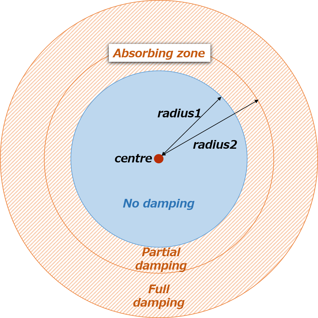
  • centre: [Required] Sphere centre location of damping
  • radius1: [Required] Inner radius at which to start damping
  • radius2: [Required] Outer radius beyond which full damping is applied
  • frequency: [Required] Frequency [Hz]
  • w: [Optional] Stencil width (default = 20)
  • Uref: [Required] Name of reference velocity field

The strength of damping is gradually increased from radius1 to radius2 and full damping is applied in the region where \(r >\) radius2. The maximum value of damping coefficient is defined as follows:

\begin{align}
\nu_{max} = w \times frequency. \tag{1} \label{eq:maxnu}
\end{align}

acousticdampingsource3

This function is only applicable for the momentum equation by default, so it needs source modifications so that it can be used in the mass and energy conservation equations as well.

An Example in 1D (Plane Wave)

Sound waves are longitudinal waves but I intentionally visualize them like the transverse waves in order to make the damping effect more visible in the following video. The damping is activated at time = 0.004s.

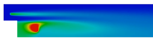
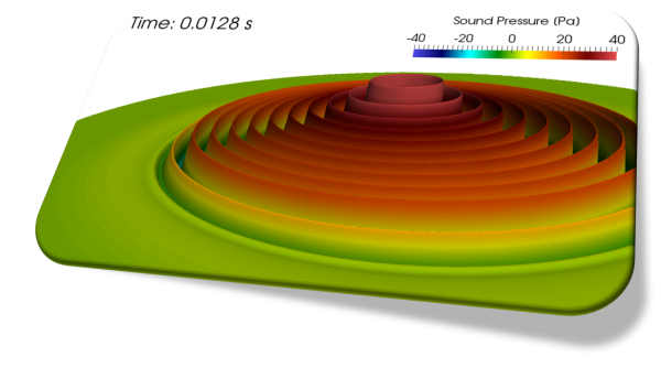
An Example in 2D (Cylindrical Wave)

Sound waves are longitudinal waves but I intentionally visualize them like the transverse waves in order to make the damping effect more visible in the following video. The damping is activated at time = 0.004s.

The amplitude gets smaller as they propagate from a sound source in contrast to the plane waves (cylindrical spreading).
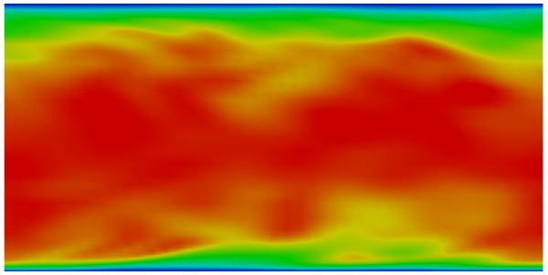
Aeolian Tone

aeoliantone

Source Code

The damping source terms added to the incompressible and compressible momentum equations are calculated by Eq. \eqref{eq:damping} in addSup function.

The profile of damping coefficient in the radial direction is calculated by the trigonometric (cosine) function in setBlendingFactor helper function.

References
  • [1] Claus Albrecht Wagner et al., Large-Eddy Simulation for Acoustics (Cambridge Aerospace Series)
  • [2] OpenFOAM® v1606+: New Solvers. Available at: https://www.openfoam.com/releases/openfoam-v1606+/solvers-and-physics.php#solvers-and-physics-acoustic-damping [Accessed: 03 May 2019].

fvOptions SemiImplicitSource

Last Updated: May 5, 2019

When we solve a partial differential equation with a source term, we must pay attention to how to treat it numerically for better convergence. The SemiImplicitSource fvOption is available in OpenFOAM so that we can handle a linearized source term in numerically stable way.

Keywords

  • Source term linearization
  • SemiImplicitSource in OpenFOAM
Source Term Linearization

If the source term under consideration is a non-linear function of a conserved variable, the linearization of it is a fundamental approach to discretizing it in the finite volume method. This topic is precisely covered in the famous book “Numerical Heat Transfer and Fluid Flow” by Suhas V. Patankar:

In Section 4.2.5, the concept of the linearization of the source term was introduced. One of the basic rules (Rule 3) required that when the source term is linearized as

\begin{equation}
S = S_C + S_P \phi_P, \tag{7.6} \label{eq:sourceTerm}
\end{equation}

the quantity \(S_P\) must not be positive. Now, we return to the topic of source-term linearization to emphasize that often source terms are the cause of divergence of iterations and that proper linearization of the source term frequently holds the key to the attainment of a converged solution.

Rule 3: Negative-slope linearization of the source term If we consider the coefficient definitions in Eqs. (3.18), it appears that, even if the neighbor coefficients are positive, the center-point coefficient \(a_P\) can become negative via the \(S_P\) term. Of course, the danger can be completely avoided by requiring that \(S_P\) will not be positive. Thus, we formulate Rule 3 as follows:

When the source term is linearized as \(\bar{S} = S_C + S_P T_P\), the coefficient \(S_P\) must always be less than or equal to zero.

Linearized Source Specification for a Scalar Field in OpenFOAM

In OpenFOAM, the linearized source terms can be specified using SemiImplicitSource fvOption. Its settings are described in the constant/fvOptions file.

  • selectionMode: [Required] Domain where the source is applied (all/cellSet/cellZone/points)
  • injectionRateSuSp: [Required] Conserved variable name and two coefficients of linearized source term

  • volumemode: [Required] Choice of how to specify the two coefficients

absolute: values are given as [variable]

specific: values are given as [variable]/\({\rm m^3}\)

Example 1. Heat Conduction with Heat Source

Let’s consider a simple 1D heat conduction problem in a solid rod with a thermal energy generation per unit volume and time \(\dot{q}_v {\rm [W/m^3]}\). In this case, the steady heat conduction equation in 1D is given by

\begin{align}
\alpha \frac{d^2 T}{d x^2} + \frac{\dot{q}_v}{\rho c} = 0. \tag{1} \label{eq:conductionEqn}
\end{align}

Here, we assume that the thermal diffusivity \(\alpha {\rm [m^2/s]}\) is constant.

We can obtain the general solution for this equation \eqref{eq:conductionEqn} by integrating it twice.

\begin{equation}
T(x) = -\frac{S_C}{2\alpha}x^2 + C_1 x + C_2, \tag{2} \label{eq:generalSolution}
\end{equation}

where \(C_1\) and \(C_2\) are integration constants and we put \(S_C {\rm [K/s]} := \dot{q}_v/\rho c\). If we assume that the temperatures at both ends of the rod are maintained at constant temperatures \(T(0) = T_1, T(L) = T_2\), we can determine the values of two integration constants as

\begin{align}
C_2 &= T_1, \tag{3} \\
C_1 &= \frac{T_2 – T_1}{L} + \frac{S_C L}{2\alpha}. \tag{4}
\end{align}

Then, the temperature distribution in the rod is expressed by the following equation:

\begin{equation}
T(x) = -\frac{S_C}{2\alpha}x^2 + \left( \frac{T_2 – T_1}{L} + \frac{S_C L}{2\alpha} \right)x + T_1. \tag{5} \label{eq:solution}
\end{equation}

t_heatsource_case1

t_heatsource

If we confine the heat source region to one-quarter of the whole region as shown in the following picture, the quadratic temperature distribution is limited to the region and the linear profile is obtained in the source free region.

t_heatsource_case2_ps2

t_heatsource_case2

t_heatsource_case2b

Example 2. Passive Scalar Transport

Explanation of fvOptions in OpenFOAM


The fvOptions functionality in OpenFOAM is flexible framework to add various source terms to the governing equations without the need to rewrite the original source code. The available options in the latest versions of OpenFOAM (v4.0 and v1606+) are listed below.

My explanations are available for the options shown in red.

I’ll extend the coverage.

Available Options

General Sources:


Pressure Gradient Sources:

  • meanVelocityForce:

    to adjust the average velocity in the whole domain or user-specified cellZone or cellSet to the desired value Ubar by adding a momentum source

  • [3.0+] directionalPressureGradientExplicitSource

Heat Exchanger Sources:


Buoyancy Sources:

  • buoyancyForce:

    to add the gravitational force term \(\rho\boldsymbol{g}\) to the momentum conservation equation in XiFoam, reactingFoam and rhoReactingFoam

  • buoyancyEnergy:

    to add the work done by gravitational force \(\rho(\boldsymbol{u} \cdot \boldsymbol{g})\) to the energy conservation equation


Porosity Sources:


Acceleration Source:


Phase Change Source:


Acoustic Damping Source:

  • [1606+] acousticDampingSource:

    to damp the acoustic waves before they reach the boundaries by adding a momentum source term in a buffer region so that the solution will not be contaminated by the reflected waves from the boundaries


Other Sources:


Solver Robustness:


Set Value:

How to Set Source Region

When specifying a source term using fvOptions in OpenFOAM, we can select the selectionMode (how to set the source region) from the following four options:

  • points
  • cellSet
  • cellZone
  • all

The meanings of these options are described in this post.


selectionMode of fvOptions in OpenFOAM

When specifying a source term using fvOptions in OpenFOAM, we can select the selectionMode (how to set the source region) from the following four options:

  • points
  • cellSet
  • cellZone
  • all

These options are defined in the cellSetOption class along with the other common parameters among the fvOptions such as timeStart and duration. Let’s check out the meaning of each option along with its source code.

selectionMode 1: points

In this case, we specify some points as shown in the following example. The source region consists of the individual cells that contain the specified points.

  • Example of description

  • Source code

selectionMode 2: cellSet

In this case, we preliminarily create a cellSet corresponding to the source region using OpenFOAM’s utilities such as setSet and specify the created cellSet name.

  • Example of description

  • Source code

selectionMode 3: cellZone

In this case, we preliminarily create a cellZone corresponding to the source region using OpenFOAM’s utilities such as setSet and specify the created cellZone name.

  • Example of description

  • Source code

selectionMode 4: all

The source region is the entire computational domain.

  • Example of description

  • Source code

fvOptions meanVelocityForce

An Example Usage of meanVelocityForce

  • fields: [Required] Name of the velocity field
  • Ubar: [Required] Desired mean velocity
  • relaxation: [Optional] Relaxation factor (default = 1.0)
  • selectionMode: [Required] Domain the source is applied (all/cellSet/cellZone/points)

The parameter name fields has been changed from fieldNames in the latest version as described in this page.

The meanVelocityForce fvOptions calculates a momentum source so that the volume averaged velocity \eqref{eq:magUbarAve} in the whole computational domain (all) or a part of domain specified using cellSet or cellZone reaches the desired mean velocity Ubar.

\begin{align}
\frac{\sum_{i}^{} \left(\frac{\bar{\boldsymbol{u}}}{|\bar{\boldsymbol{u}}|} \cdot \boldsymbol{u}_i \right)V_i}{\sum_{i}^{} V_i}, \tag{1} \label{eq:magUbarAve}
\end{align}
where the summation is over the cells that belong to the user-specified domain, \(\bar{\boldsymbol{u}}\) is Ubar, \(\boldsymbol{u}_i\) is the velocity in the i-th cell and \(V_i\) is the volume of the i-th cell.

patchMeanVelocityForce

The patchMeanVelocityForce fvOptions is also available to specify the desired mean velocity on a patch instead of the volumetric average \eqref{eq:magUbarAve}.

Tutorial
Source Code

In the case of pimpleFoam, we can find three lines related to the fvOptions as shown in the following code (UEqn.H):

In what follows, we will take a closer look at each of three highlighted lines when the meanVelocityForce fvOptions is used. The source files of this class are in src/fvOptions/sources/derived/meanVelocityForce.

  • l. 11

The addSup function is called from l.11 in UEqn.H when discretizing the momentum equation and source term Su is added to the equation.

  • l. 17

The constrain function is called from l.17 in UEqn.H. The if loop is true in the first iteration and else loop is executed for the other iterations to initialize and update the volScalarField defined as the reciprocal of the diagonal coefficients.

  • l. 23

As the average velocity magUbarAve \eqref{eq:magUbarAve} reaches a user-specified value Ubar, the pressure gradient increment dGradP_ needed to adjust the average velocity converges to 0.