Last Updated: May 5, 2019
When we solve a partial differential equation with a source term, we must pay attention to how to treat it numerically for better convergence. The SemiImplicitSource fvOption is available in OpenFOAM so that we can handle a linearized source term in numerically stable way.
Keywords
- Source term linearization
- SemiImplicitSource in OpenFOAM
| Source Term Linearization |
If the source term under consideration is a non-linear function of a conserved variable, the linearization of it is a fundamental approach to discretizing it in the finite volume method. This topic is precisely covered in the famous book “Numerical Heat Transfer and Fluid Flow” by Suhas V. Patankar:
In Section 4.2.5, the concept of the linearization of the source term was introduced. One of the basic rules (Rule 3) required that when the source term is linearized as
\begin{equation}
S = S_C + S_P \phi_P, \tag{7.6} \label{eq:sourceTerm}
\end{equation}the quantity \(S_P\) must not be positive. Now, we return to the topic of source-term linearization to emphasize that often source terms are the cause of divergence of iterations and that proper linearization of the source term frequently holds the key to the attainment of a converged solution.
Rule 3: Negative-slope linearization of the source term If we consider the coefficient definitions in Eqs. (3.18), it appears that, even if the neighbor coefficients are positive, the center-point coefficient \(a_P\) can become negative via the \(S_P\) term. Of course, the danger can be completely avoided by requiring that \(S_P\) will not be positive. Thus, we formulate Rule 3 as follows:
When the source term is linearized as \(\bar{S} = S_C + S_P T_P\), the coefficient \(S_P\) must always be less than or equal to zero.
| Linearized Source Specification for a Scalar Field in OpenFOAM |
In OpenFOAM, the linearized source terms can be specified using SemiImplicitSource fvOption. Its settings are described in the constant/fvOptions file.
|
1 2 3 4 5 6 7 8 9 10 11 12 13 14 15 16 17 18 19 20 21 22 23 24 25 26 27 28 29 30 31 32 33 34 35 36 |
/*--------------------------------*- C++ -*----------------------------------*\ | ========= | | | \\ / F ield | OpenFOAM: The Open Source CFD Toolbox | | \\ / O peration | Version: dev | | \\ / A nd | Web: www.OpenFOAM.org | | \\/ M anipulation | | \*---------------------------------------------------------------------------*/ FoamFile { version 2.0; format ascii; class dictionary; location "constant"; object fvOptions; } // * * * * * * * * * * * * * * * * * * * * * * * * * * * * * * * * * * * * * // heatSource { type scalarSemiImplicitSource; active true; scalarSemiImplicitSourceCoeffs { selectionMode all; // all, cellSet, cellZone, points cellSet c1; volumeMode specific; // absolute; injectionRateSuSp { T (0.1 0); } } } // ************************************************************************* // |
- selectionMode: [Required] Domain where the source is applied (all/cellSet/cellZone/points)
- injectionRateSuSp: [Required] Conserved variable name and two coefficients of linearized source term
|
1 2 3 4 |
injectionRateSuSp { variable_name (Sc Sp); } |
- volumemode: [Required] Choice of how to specify the two coefficients
– absolute: values are given as [variable]
– specific: values are given as [variable]/\({\rm m^3}\)
| Example 1. Heat Conduction with Heat Source |
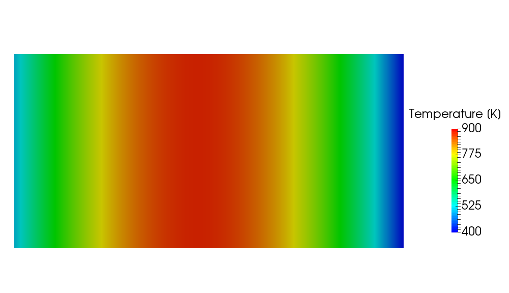
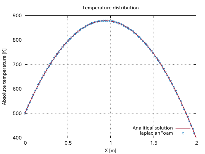
Let’s consider a simple 1D heat conduction problem in a solid rod with a thermal energy generation per unit volume and time \(\dot{q}_v {\rm [W/m^3]}\). In this case, the steady heat conduction equation in 1D is given by
\begin{align}
\alpha \frac{d^2 T}{d x^2} + \frac{\dot{q}_v}{\rho c} = 0. \tag{1} \label{eq:conductionEqn}
\end{align}
Here, we assume that the thermal diffusivity \(\alpha {\rm [m^2/s]}\) is constant.
We can obtain the general solution for this equation \eqref{eq:conductionEqn} by integrating it twice.
\begin{equation}
T(x) = -\frac{S_C}{2\alpha}x^2 + C_1 x + C_2, \tag{2} \label{eq:generalSolution}
\end{equation}
where \(C_1\) and \(C_2\) are integration constants and we put \(S_C {\rm [K/s]} := \dot{q}_v/\rho c\). If we assume that the temperatures at both ends of the rod are maintained at constant temperatures \(T(0) = T_1, T(L) = T_2\), we can determine the values of two integration constants as
\begin{align}
C_2 &= T_1, \tag{3} \\
C_1 &= \frac{T_2 – T_1}{L} + \frac{S_C L}{2\alpha}. \tag{4}
\end{align}
Then, the temperature distribution in the rod is expressed by the following equation:
\begin{equation}
T(x) = -\frac{S_C}{2\alpha}x^2 + \left( \frac{T_2 – T_1}{L} + \frac{S_C L}{2\alpha} \right)x + T_1. \tag{5} \label{eq:solution}
\end{equation}
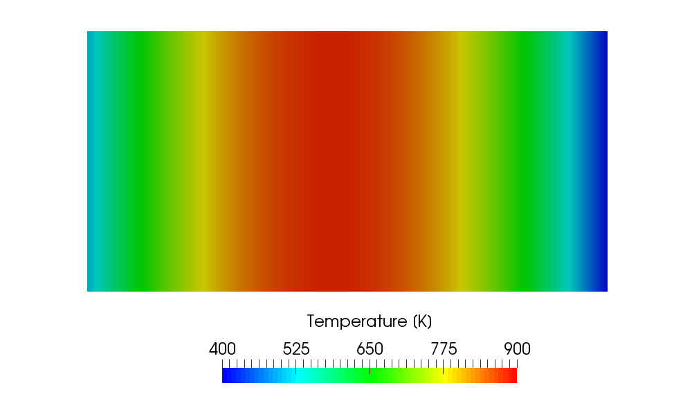
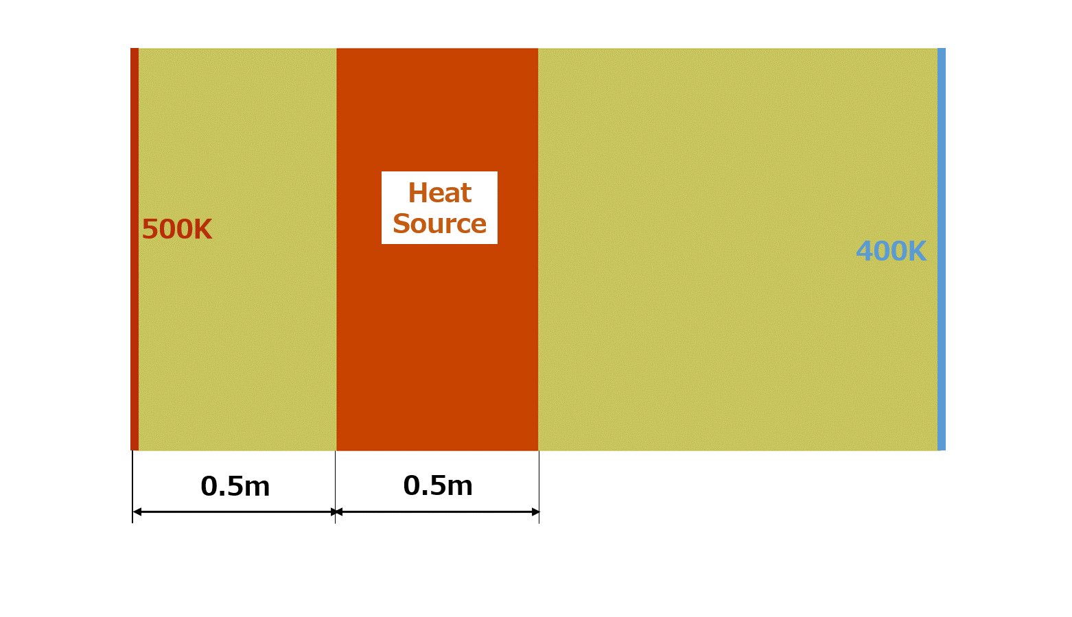
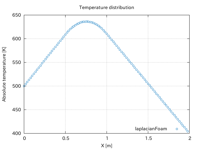
If we confine the heat source region to one-quarter of the whole region as shown in the following picture, the quadratic temperature distribution is limited to the region and the linear profile is obtained in the source free region.

| Example 2. Passive Scalar Transport |