Bandwidth, Profile and Frontwidth of Matrix

When we discretize the partial differential equations using the Finite Volume Method (FVM), we get sets of linear algebraic equations with large sparse coefficient matrices that are solved using iterative or direct methods. There is renumberMesh utility in OpenFOAM that is used to reduce the bandwidth of the coefficient matrices by renumbering the cell label list.

The bandwidth is not a special term in OpenFOAM but it is a general concept in the field of solving linear systems of equations. In this blog post, I will try to give a description of it and other important terms such as profile and frontwidth.

Keywords: bandwidth, profile, frontwidth, renumberMesh

Definitions of bandwidth, profile and frontwidth

The definitions of these terms are clearly described in [1]. Let \(A\) be an \(N\) by \(N\) matrix with symmetric zero-nonzero structure, i.e. , \(a_{ij} \neq 0\) if and only if \(a_{ji} \neq 0\).

The \(i\)-th bandwidth of \(A\) is:

\begin{align}
\beta_i(A) = i \; – \; {\rm min}\{ j \; | \; a_{ij} \neq 0\}. \tag{1} \label{eq:ithBandwidth}
\end{align}

The bandwidth of \(A\) is defined by

\begin{align}
\beta = \beta(A) &= {\rm max} \{ \beta_i(A) \; | \; 1 \leq i \leq N\} \\
&= {\rm max} \{ |i-j| \; | \; a_{ij} \neq 0 \}. \tag{2} \label{eq:Bandwidth}
\end{align}

The quantity \(|Env(A)|\) is called the profile or the envelope size of \(A\), and is defined by:

\begin{align}
|Env(A)| = \sum_{i=1}^{N} \beta_i(A). \tag{4} \label{eq:Profile}
\end{align}

Another quantity called frontwidth is defined by the number of rows of the envelope of \(A\) which intersect column \(i\).

\begin{align}
\omega_i(A) = \{ k \; | \; k > i \; and \; \exists l \leq i \; s.t. \; a_{kl} \neq 0 \} \tag{5} \label{eq:frontwidth}
\end{align}

To estimate factorization time, a quantity called root mean square frontwidth is introduced by [2]. This quantity is given by:

\begin{align}
f = \sqrt{\frac{1}{N} \left( \sum_{i=1}^{N} \omega_i^2 \right)}. \tag{8} \label{eq:rmsFrontwidth}
\end{align}

Output of renumberMesh utility

When the renumberMesh utility is executed, the following data is reported to the screen.

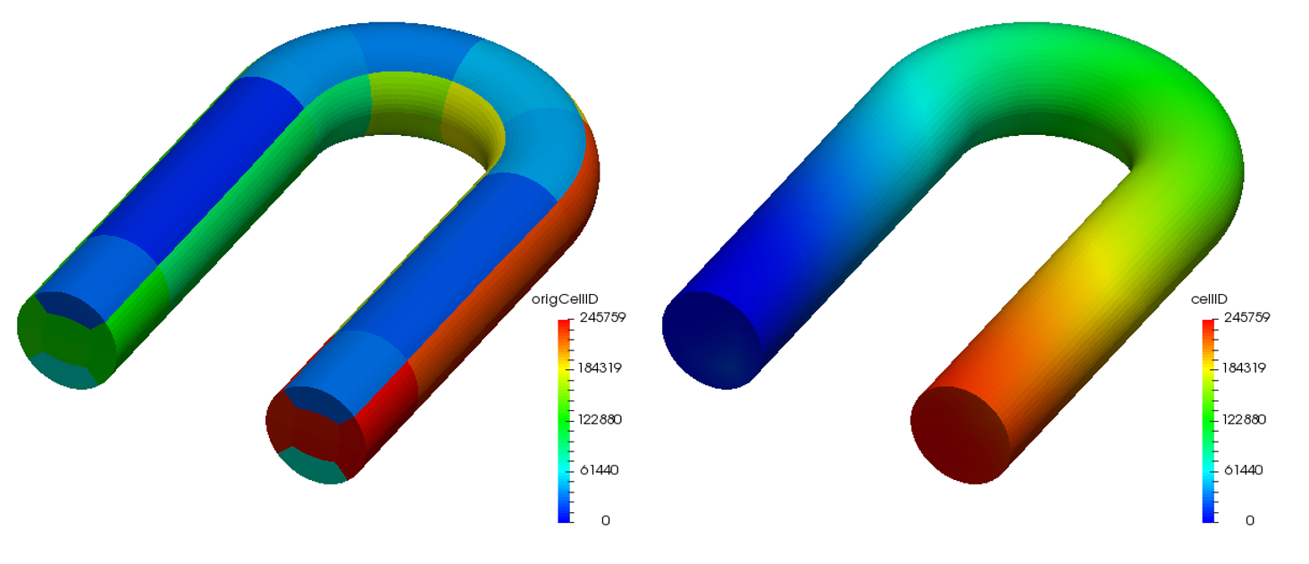
Here, the band, profile and rms frontwidth correspond to \eqref{eq:Bandwidth}, \eqref{eq:Profile} and \eqref{eq:rmsFrontwidth}, respectively. We can confirm that they all decreased after renumbering the cell label using the Cuthill-McKee (CM) algorithm. The distributions of cell labels are visually compared between before and after reordering operations in Figure 1.

celllabel
Fig. 1 (Left) Before reordering, (Right) After reordering.
Source code of renumberMesh utility

The getBand function is called from the main function. The variables band, profile and rmsFrontwidth represent \eqref{eq:Bandwidth}, \eqref{eq:Profile} and \eqref{eq:rmsFrontwidth}, respectively.

References

Introduction to laplacianFoam and simple validation calculation


In this blog post, I will try to give a description of the governing equation of the laplacianFoam in OpenFOAM that solves a simple Laplace equation, e.g. for thermal diffusion in a solid.

Governing Equation

The heat conduction equation is given by the following equation:

\begin{align}
\frac{\partial T}{\partial t} = \frac{1}{\rho c_p} \nabla \cdot \left(k \nabla T\right) + \frac{q}{\rho c_p}, \tag{1} \label{eq:conductionEqn}
\end{align}

where \(T\;{\rm [ K]}\) is the absolute temperature field, \(\rho\;{\rm [kg/m^3]}\) is the density field, \(q\;{\rm [W/m^3]}\) is the rate of energy generation per unit volume, \(k\;{\rm [W/(m\cdot K)]}\) is the thermal conductivity and \(c_p\;{\rm [J/(kg\cdot K)]}\) is the specific heat at constant pressure.

If the heat capacity \(\rho c_p\) is spatially uniform, the Eq. \eqref{eq:conductionEqn} can be transformed into the following form irrespective of whether the thermal conductivity \(k\) is spatially uniform or not:

\begin{align}
\frac{\partial T}{\partial t} = \nabla \cdot \left(\alpha \nabla T\right) + \frac{q}{\rho c_p}, \tag{2} \label{eq:conductionEqn2}
\end{align}

where \(\alpha = k/\rho c_p\;{\rm [m^2/s]}\) is the thermal diffusivity.

The laplacianFoam (in OpenFOAM-4.x and earlier versions) doesn’t consider the heat generation and the implemented equation is

\begin{align}
\frac{\partial T}{\partial t} = \nabla \cdot \left(\alpha \nabla T\right), \tag{3} \label{eq:laplacianFoam}
\end{align}

but the solver in the latest development version supports the fvOptions so that we can solve \eqref{eq:conductionEqn2} and specify a volumetric heat source.

We can find the Eq. \eqref{eq:conductionEqn2} solved in laplacianFoam.C.

The variable DT represents the thermal diffusivity \(\alpha\) and it is specified in the constant/transportProperties file.

Comparison with Analytical Solution

We consider the steady state problem of source-free heat conduction in a concentric cylinder whose inner and outer walls are maintained at constant temperature of 400 K and 300 K respectively. This problem can be analytically solved and the following relation holds for the temperature distribution in the radial direction \(T(r)\):

\begin{align}
\frac{T_1 – T(r)}{T_1 – T_2} = \frac{\ln{(r/r_1)}}{\ln{(r_2/r_1)}}, \tag{4} \label{eq:cylinderT}
\end{align}

where the subscripts 1 and 2 indicate the values at the inner and outer walls respectively shown in Figure 1.

conduction_pb1
Fig. 1 Problem setting

The temperature distribution obtained using laplacianFoam is shown in Figure 2 and the comparison between the numerical and analytical solutions is shown in Figure 3. The agreement with the analytical solution is good.

Fig. 2
Fig. 2 Temperature distribution
conduction_pb1_comparison
Fig. 3 Comparison of numerical and analytical solutions
Introduction of Source Term

In the next post, I’ll deal with a simple example case to introduce how to specify a heat generation source term in laplacianFoam using the fvOptions functionality (scalarSemiImplicitSource).

t_heatsource

Function Objects – histogram


OpenFOAM Version:
OpenFOAM-4.x

Settings of histogram

Histogram

You can create a picture as shown below using Gnuplot with the input file generated by OpenFOAM. I replaced “with lines” with “with boxes” in the input command file to create this picture.

histgram

In the above picture, the first bin represents the following volume fraction:

\begin{align}
\frac{\sum_{celli}^{} \left( V_{celli}:\;300 \leq T_{celli} < 301\right)}{\sum_{celli}^{} \left( V_{celli}:\;min \leq T_{celli} < max\right)},
\end{align}

where \(V\) is the cell volume.

buoyantPimpleFoam and buoyantSimpleFoam in OpenFOAM


In this blog post, I will try to give a description of the governing equations of the following solvers in OpenFOAM for buoyant, turbulent flow of compressible fluids:

  • buoyantPimpleFoam (Transient solver)
  • buoyantSimpleFoam (Steady-state solver)

The solvers in OpenFOAM are named properly and comprehensibly so that the users can guess the meanings from their names 🙂

Mass Conservation

The mass conservation (continuity) equation of buoyantPimpleFoam is given by the following equation:

\begin{align}
\frac{\partial \rho}{\partial t} + \nabla \cdot \left( \rho \boldsymbol{u} \right) = 0, \tag{1} \label{eq:mass}
\end{align}
where \(\boldsymbol{u}\) is the velocity field and \(\rho\) is the density field. For the steady-state solver, the time derivative term is omitted.

Momentum Conservation

The momentum conservation equation of buoyantPimpleFoam is given by the following equation:

\begin{align}
\frac{\partial \left(\rho \boldsymbol{u} \right)}{\partial t} + \nabla \cdot \left(\rho\boldsymbol{u}\boldsymbol{u}\right) = &-\nabla p + \rho \boldsymbol{g} + \nabla \cdot \left(2 \mu_{eff} D \left( \boldsymbol{u} \right) \right) \\
&-\nabla \left( \frac{2}{3}\mu_{eff}\left(\nabla \cdot \boldsymbol{u} \right) \right), \tag{2} \label{eq:momentum}
\end{align}

where \(p\) is the static pressure field and \(\boldsymbol{g}\) is the gravitational acceleration. The effective viscosity \(\mu_{eff}\) is the sum of the molecular and turbulent viscosity and the rate of strain (deformation) tensor \(D\left(\boldsymbol{u}\right)\) is defined as \(D\left(\boldsymbol{u}\right) = \frac{1}{2}\left( \nabla \boldsymbol{u} + \left(\nabla \boldsymbol{u}\right)^{T} \right)\). As is the case in the continuity equation, the time derivative term is omitted in buoyantSimpleFoam.

In terms of the implementation in OpenFOAM, the pressure gradient and gravity force terms are rearranged in the following form:

\begin{align}
-\nabla p + \rho \boldsymbol{g}
&= -\nabla \left( p_{rgh} + \rho \boldsymbol{g} \cdot \boldsymbol{r} \right) + \rho \boldsymbol{g} \tag{3a}\\
&= -\nabla p_{rgh} – \left( \boldsymbol{g} \cdot \boldsymbol{r} \right) \nabla \rho \:- \rho \boldsymbol{g} + \rho \boldsymbol{g} \tag{3b} \\
&= -\nabla p_{rgh} – \left( \boldsymbol{g} \cdot \boldsymbol{r} \right) \nabla \rho, \tag{3c} \label{eq:prgh}
\end{align}

where \(p_{rgh} = p \;- \rho \boldsymbol{g} \cdot \boldsymbol{r}\) and \(\boldsymbol{r}\) is the position vector.

In the above code, MRF stands for Multiple Reference Frame, which is one method for solving the problems including the rotating parts with the static mesh. This option is activated if constant/MRFProperties file exists. The line 11(fvOptions(rho, U)) is to add the user-specific source terms using fvOptions functionality.

Energy Conservation

We can choose either internal energy \(e\) or enthalpy \(h\) as the energy solution variable [3]. This selection is made according to energy keyword in thermophysicalProperties file.

For each variable, the energy conservation equations of buoyantPimpleFoam are given by the following equations:

  • Enthalpy (sensibleEnthalpy)

\begin{align}
&\frac{\partial \left(\rho h \right)}{\partial t} + \nabla \cdot \left( \rho \boldsymbol{u} h \right) + \frac{\partial \left(\rho K \right)}{\partial t} + \nabla \cdot \left( \rho \boldsymbol{u} K \right) -\frac{\partial p}{\partial t} \\
&= \nabla \cdot \left( \alpha_{eff} \nabla h \right) + \rho \boldsymbol{u} \cdot \boldsymbol{g} \tag{4} \label{eq:energyH}
\end{align}

  • Internal energy (sensibleInternalEnergy)

\begin{align}
&\frac{\partial \left(\rho e \right)}{\partial t} + \nabla \cdot \left( \rho \boldsymbol{u} e \right) + \frac{\partial \left(\rho K \right)}{\partial t} + \nabla \cdot \left( \rho \boldsymbol{u} K \right) + \nabla \cdot \left( p \boldsymbol{u} \right) \\
&= \nabla \cdot \left( \alpha_{eff} \nabla e \right) + \rho \boldsymbol{u} \cdot \boldsymbol{g} \tag{5} \label{eq:energyE}
\end{align}

where \(K \equiv |\boldsymbol{u}|^2/2\) is kinetic energy per unit mass and the enthalpy per unit mass \(h\) is the sum of the internal energy per unit mass \(e\) and the kinematic pressure \(h \equiv e + p/\rho\). We can get the following relations from this definition:
\begin{align}
\frac{\partial \left(\rho e \right)}{\partial t} = \frac{\partial \left(\rho h \right)}{\partial t} \;-\; \frac{\partial p}{\partial t}, \tag{6a} \\
\nabla \cdot \left( \rho \boldsymbol{u} e \right) = \nabla \cdot \left( \rho \boldsymbol{u} h \right) \;-\; \nabla \cdot \left( p \boldsymbol{u} \right). \tag{6b}
\end{align}

The effective thermal diffusivity \(\alpha_{eff}/\rho\) is the sum of laminar and turbulent thermal diffusivities:

\begin{align}
\alpha_{eff} = \frac{\rho \nu_t}{Pr_t} + \frac{\mu}{Pr} = \frac{\rho \nu_t}{Pr_t} + \frac{k}{c_p}, \tag{7} \label{eq:alphaEff}
\end{align}

where \(k\) is the thermal conductivity, \(c_p\) is the specific heat at constant pressure, \(\mu\) is the dynamic viscosity, \(\nu_t\) is the turbulent (kinematic) viscosity, \(Pr\) is the Prandtl number and \(Pr_t\) is the turbulent Prandtl number. The expression of the laminar thermal diffusivity changes depending on the selected thermodynamics package. As is the case in the momentum equation, the time derivative terms are omitted in buoyantSimpleFoam.

The line 21 represents the contributions from the radiative heat transfer. The effective thermal diffusivity \(\alpha_{eff}\) \eqref{eq:alphaEff} is calculated in heThermo.C:

When solving for enthalpy \(h\), the pressure-work term \(dp/dt\) can be excluded by setting the dpdt option to no in thermophysicalProperties file [3]. The volScalarField \(dp/dt\) is defined and uniformly initialized to zero in createFields.H and updated in pEqn.H if this option is activated.

When the mesh is static, the fvc::absolute function does nothing as shown below:

References

[1] Energy Equation in OpenFOAM | CFD Direct
[2] OpenFOAM User Guide: 7.1 Thermophysical models | CFD Direct
[3] OpenFOAM 2.2.0: Thermophysical Modelling

Postprocessing with foamCalc utility


After the simulation has finished, you can do simple calculation, such as addition and subtraction, with the field data using foamCalc utility. The source code is located in the following directories:

  • applications/utilities/postProcessing/foamCalc
  • src/postProcessing/foamCalcFunctions.
components
 $ foamCalc components U -latestTime 

This example is to generate three component files Ux, Uy and Uz (volScalarField) from volVectorField U only at the latest time directory.

mag
 $ foamCalc mag U 

This example is to generate velocity magnitude field \(|\boldsymbol{U}|\) file magU at every existing time directory.

magSqr
 $ foamCalc magSqr U 

This example is to generate magnitude squared field \(|\boldsymbol{U}|^2\) file magSqrU at every existing time directory.

addSubtract
 $ foamCalc addSubtract T subtract -value 273.15 -resultName Tdeg -time 5000 

This example is to convert the temperature unit from Kelvin to degrees at time 5000. The generated file name can be specified using –resultName option.

div
 $ foamCalc div phi 

This example is to calculate the divergence of the flux field phi for the estimation of the continuity error of each cell for incompressible flow.

interpolate
 $ foamCalc interpolate T -latestTime 

This example it to generate surfaceScalarField interpolateT from volScalarField T using the interpolation scheme specified in the system/fvSchemes file.

Conduction, convection and radiation in OpenFOAM (Under construction)

This page is under construction. I will update by adding a description of each solver and model.

Conduction

flangeT

Convection
Conduction + Convection (Conjugate Heat Transfer)
  • chtMultiRegionSimpleFoam (Steady)
  • chtMultiRegionFoam (Transient)
+ Radiation

All the above solvers but laplacianFoam are able to deal with the radiative heat transfer. There are the following five (virtually four) models available in OpenFOAM. Their source code is located in src/thermophysicalModels/radiation/radiationModels and we can see the brief descriptions in the header file of each radiation class.

  • P1

Keywords: optical thickness [2]

  • fvDOM (Finite Volume Discrete Ordinates Method)

  • viewFactor

  • opaqueSolid

  • none

The settings of the radiation models are described in constant/radiationProperties file.

References

Solvers for heat transfer problems in OpenFOAM – buoyantBoussinesqPimpleFoam


There are several solvers for solving the heat transfer problems in OpenFOAM. In this post, I will try to give a description of how to derive the governing equations of the following two solvers:

  • buoyantBoussinesqSimpleFoam
  • buoyantBoussinesqPimpleFoam

In the presence of gravity body force, the mass and momentum conservation equations are:

\begin{align}
\frac{\partial \rho}{\partial t} + \nabla \cdot \left(\rho \boldsymbol{u}\right) = 0, \tag{1} \label{eq:massEqn}
\end{align}

\begin{align}
\frac{\partial \left(\rho \boldsymbol{u} \right)}{\partial t} + \nabla \cdot \left(\rho\boldsymbol{u}\boldsymbol{u}\right) = &-\nabla p + \rho \boldsymbol{g} + \nabla \cdot \left(2 \mu_{eff} D \left( \boldsymbol{u} \right) \right) \\
&-\nabla \left( \frac{2}{3}\mu_{eff}\left(\nabla \cdot \boldsymbol{u} \right) \right), \tag{2} \label{eq:momEqn}
\end{align}

where \(\boldsymbol{u}\) is the velocity field, \(p\) is the pressure field, \(\rho\) is the density field, and \(\boldsymbol{g}\) is the gravitational acceleration. The effective viscosity \(\mu_{eff}\) is the sum of the molecular and turbulent viscosity and the rate of strain tensor \(D\left(\boldsymbol{u}\right)\) is defined as \(D\left(\boldsymbol{u}\right) = \frac{1}{2}\left( \nabla \boldsymbol{u} + \left(\nabla \boldsymbol{u}\right)^{T} \right)\).

If both density and gravitational acceleration are constant, the gravitational force can be expressed in terms of gradient:

\begin{align}
\rho \boldsymbol{g} = \nabla \left( \rho \boldsymbol{g} \cdot \boldsymbol{r} \right), \tag{3} \label{eq:Fgravity}
\end{align}

where \(\boldsymbol{r}\) is the position vector, so that the pressure gradient and gravity force can be lumped together as shown in the following equation:

\begin{align}
\nabla p \;-\; \rho \boldsymbol{g} = \nabla \left( p \;-\; \rho \boldsymbol{g} \cdot \boldsymbol{r} \right). \tag{4} \label{eq:conversion}
\end{align}

Boussinesq approximation

Now we consider the case when the density is not constant. The Boussinesq approximation is valid when the variation of the density induced by the temperature change is small, as Ferziger and Peric (2001, pp.14-15) states that:

In flows accompanied by heat transfer, the fluid properties are normally functions of temperature. The variations may be small and yet be the cause of the fluid motion. If the density variation is not large, one may treat the density as constant in the unsteady and convection terms, and treat it as variable only in the gravitational term. This is called the Boussinesq approximation.

Hereafter, we denote the reference density by \(\rho_0\) at the reference temperature \(T_0\). If we replace \(\rho\) by \(\rho_0\) in the Eq.\eqref{eq:massEqn}\eqref{eq:momEqn} except for the gravitational term, then we get:

\begin{align}
\nabla \cdot \boldsymbol{u} = 0, \tag{5} \label{eq:massEqn2}
\end{align}

\begin{align}
\frac{\partial \left(\rho_0 \boldsymbol{u} \right)}{\partial t} + \nabla \cdot \left(\rho_0\boldsymbol{u}\boldsymbol{u}\right) = -\nabla p + \rho \boldsymbol{g} + \nabla \cdot \left(2 \mu_{eff} D \left( \boldsymbol{u} \right) \right). \tag{6} \label{eq:momEqn2}
\end{align}

Then divide both sides of Eq.\eqref{eq:momEqn2} by \(\rho_0\) and we get:

\begin{align}
\frac{\partial \boldsymbol{u}}{\partial t} + \nabla \cdot \left(\boldsymbol{u}\boldsymbol{u}\right) = -\frac{1}{\rho_0} \left( \nabla p \;-\; \rho\boldsymbol{g} \right) + \nabla \cdot \left(2 \nu_{eff} D \left( \boldsymbol{u} \right) \right). \tag{7} \label{eq:momEqn3}
\end{align}

Here, the density \(\rho\) in the gravitational term is expressed by the linear function of the temperature \(T\):

\begin{align}
\rho \approx \rho_0\left[ 1 \;-\; \beta\left( T \;-\; T_0 \right) \right]. \tag{8} \label{eq:rhoEqn}
\end{align}

This relation is derived from the definition of the volumetric thermal expansion coefficient \(\beta\):

\begin{align}
\beta \equiv -\frac{1}{\rho}\frac{\partial \rho}{\partial T}
\approx -\frac{1}{\rho_0}\frac{\rho \;-\; \rho_0}{T \;-\; T_0}. \tag{9} \label{eq:beta}
\end{align}

We have to know when these approximations are valid. Ferziger and Peric (2001, p.15) states that:

This approximation introduces errors of the order of 1% if the temperature differences are below e.g. 2℃ for water and 15℃ for air. The error may be more substantial when temperature differences are larger; the solution may even be qualitatively wrong.

If temperature differences are larger, we should use buoyantSimpleFoam or buoyantPimpleFoam without Boussinesq approximation.

In terms of the implementation, the pressure gradient and gravity force terms are rearranged in the following form:

\begin{align}
&-\nabla \left(\frac{p}{\rho_0}\right) + \left(\frac{\rho}{\rho_0}\right)\boldsymbol{g} \\
=&-\nabla \left(\frac{p \;- \rho \boldsymbol{g} \cdot \boldsymbol{r}}{\rho_0} + \frac{\rho \boldsymbol{g} \cdot \boldsymbol{r}}{\rho_0} \right) + \left(\frac{\rho}{\rho_0}\right)\boldsymbol{g} \tag{10a}\\
=&-\nabla p_{rgh} – \left( \boldsymbol{g} \cdot \boldsymbol{r} \right) \nabla \left(\frac{\rho}{\rho_0}\right), \tag{10b} \label{eq:final}
\end{align}

where we define a new variable \(p_{rgh} = \left(p-\rho\boldsymbol{g}\cdot\boldsymbol{r}\right)/\rho_0\) and finally we get:

\begin{align}
\frac{\partial \boldsymbol{u}}{\partial t} + \nabla \cdot \left(\boldsymbol{u}\boldsymbol{u}\right) =\; &- \nabla p_{rgh} – \left( \boldsymbol{g} \cdot \boldsymbol{r} \right) \nabla \left(\frac{\rho}{\rho_0}\right) \\ &+ \nabla \cdot \left(2 \nu_{eff} D \left( \boldsymbol{u} \right) \right). \tag{11} \label{eq:momEqn4}
\end{align}

This momentum equation \eqref{eq:momEqn4} is implemented in UEqn.H as shown in the following code:

The Eq. \eqref{eq:final} is calculated using the fvc::reconstruct function from the face flux fields and the variable rhok is defined in createFields.H as \(\rho/\rho_0\):

Reference

[1] Joel H. Ferziger and Milovan Peric (2001): Computational Methods for Fluid Dynamics

Please wait till the next update!

reconstruct 演算子について #2

前回の投稿 の続きとして,reconstruct 演算子をもう少し詳しく見ていきます.前回の投稿で掲載した reconstruct 演算子の定義式は,数式では次式\eqref{eq:reconstruct}のように表現できます.

$$ reconstruct(ssf) = \left(\sum_{f}^{}{\left({\bf n}_f \otimes {\bf S}_f\right)} \right)^{-1}\left(\sum_{f}^{} {\bf n}_f ssf\right) \tag{1} \label{eq:reconstruct} $$

ここで,\({\bf n}_f\) は,フェイスの単位法線ベクトルを,\({\bf S}_f\left(=|{\bf S}_f|{\bf n}_f\right)\) は,フェイスの面積を大きさとし,向きが \({\bf n}_f\) と等しい法線ベクトルをそれぞれ表します.また,surfaceSum 演算子は,各セルにおいてそのセルのフェイスの値の総和を計算します(fvcSurfaceIntegrate.C).

事前準備

\eqref{eq:reconstruct}式中で使用されている2つのベクトル \(\bf a\) と \(\bf b\) の二項積\(\otimes\) (dyadic product) は次式\eqref{eq:dyad}のように計算されます.

$$ {\bf a} \otimes {\bf b} = \left(
\begin{array}{ccc}
a_1b_1 & a_1b_2 & a_1b_3 \\
a_2b_1 & a_2b_2 & a_2b_3 \\
a_3b_1 & a_3b_2 & a_3b_3
\end{array}
\right) \tag{2} \label{eq:dyad} $$

この二項積とベクトル \(\bf c\) との積を計算すると,次式\eqref{eq:D}のように変形できます.

\begin{align} \left({\bf a} \otimes {\bf b}\right) {\bf c} &= \left(
\begin{array}{ccc}
a_1b_1 & a_1b_2 & a_1b_3 \\
a_2b_1 & a_2b_2 & a_2b_3 \\
a_3b_1 & a_3b_2 & a_3b_3
\end{array}
\right)\left(
\begin{array}{c}
c_1 \\
c_2 \\
c_3
\end{array}
\right) \\
& = {\bf a}\left({\bf b} \cdot {\bf c}\right) \tag{3} \label{eq:D}
\end{align}

準備は以上です.

本題

では本題です.関係式\eqref{eq:D}を使用して,reconstruct 演算子を調べていきます.ここで,\eqref{eq:reconstruct}式中の以下の行列の部分を

$$ D \equiv \sum_{f}^{}{\left({\bf n}_f \otimes {\bf S}_f\right)} \tag{4} \label{eq:Dop} $$

として,密度 \(\rho\) の勾配 \(\nabla \rho\) にこれを作用させてみます.

\begin{align}
D \nabla \rho &= \sum_{f}^{} {\left({\bf n}_f\left({\bf S}_f \cdot \nabla \rho \right)\right)} \tag{5a}\\
&= \sum_{f}^{} {\left({\bf n}_f\left(|{\bf S}_f|{\bf n}_f \cdot \nabla \rho \right)\right)} \tag{5b}\\
&\approx \sum_{f}^{} {\left({\bf n}_f\left(|{\bf S}_f|{\bf n}_f \cdot \left(\nabla \rho\right)_f \right)\right)} \tag{5c}\\
& = \sum_{f}^{} {\left({\bf n}_f\left(|{\bf S}_f|snGrad\left(\rho\right)_f \right)\right)} \tag{5d} \label{eq:conversion}
\end{align}

ここで,1つ目の変形で関係式\eqref{eq:D}を使用しています.そして,3つ目の変形に近似が含まれています.これを\eqref{eq:reconstruct}式に合わせて書き直すと,次式が得られます.
$$ \nabla \rho \approx D^{-1}\left(\sum_{f}^{} {\left({\bf n}_f|{\bf S}_f|snGrad\left(\rho\right)_f \right)}\right) \tag{6} \label{eq:final} $$

参考資料

[1] CFD Online Forums: fvc::reconstruct( ) algorithm

reconstruct 演算子について #1

OpenFOAM のソースコードを眺めていると,fvc::reconstruct という演算子を目にします.例えば,buoyantSimpleFoam の UEqn.H ではこの演算子が下記のように使用されています.

これは,具体的にどのような演算を行っているのでしょうか?こんな時は,ソースコードを確認しましょう.ソースコードを参照して実装方法をすぐに確認できるのが,オープンソースの1つのメリットですね.この演算子のソースファイルは,fvcReconstruct.C です.このファイルの 76 行目に演算の定義が記述されています.

私は一見しただけでは何を行っているのか分かりませんでした.ヘッダーファイル fvcReconstruct.H も確認してみます.

冒頭の Description の項目に,Reconstruct volField from a face flux field という記述があります.最初に挙げた buoyantSimpleFoam での使用例を確認すると,fvc::reconstruct(引数) の引数は,フェイス(セル界面)で値をもっています(face flux field).具体的には,

  • snGrad(rho) は,フェイスの法線方向の密度の勾配を,
  • mesh.magSf() は,フェイスの面積を

それぞれ計算するので,両方とも値はフェイスで保持しています.この例では,OpenFOAM の用語を使用すると,surfaceScalarField を引数をとして受け取り,セル中心で値をもつ volVectorField を返しています.

次回予告

次回の投稿では,簡単な例でこの演算子を書き下して,数式を使用した説明にチャレンジしたいと思います.最終的には,重力のような体積力を考慮した計算において,圧力の変数として \(p\) ではなく \(p_{rgh}\) を使用することの数値計算上の利点に関する説明につなげられたらと考えています.では!

fixedFluxPressure 境界条件


OpenFOAM で自然対流を伴う熱流体計算や混相流 (Multiphase) 計算のように重力を考慮する計算を行う場合には,流れ場を表す変数として静圧 \(p\) そのものではなく,次式\eqref{eq:prgh}で定義される変数 \(p_{rgh}\) を使用します.

\begin{equation}
p_{rgh} = p\;-\;\rho{\bf g} \cdot {\bf x} \tag{1} \label{eq:prgh}
\end{equation}

ここで,\(\rho\) は流体の密度を,\(\boldsymbol{g}\) は重力加速度ベクトルを,\(\boldsymbol{x}\) は位置ベクトルをそれぞれ表します.OpenFOAM で p_rgh と表されるこの変数の境界条件として,以前は,buoyantPressure 条件が使用されていましたが,v2.3 以降では,fixedFluxPressure 条件が使用されています.今回の投稿では,この2つの境界条件について取り上げます.

fixedFluxPressure 境界条件

セル界面の流速 \(\boldsymbol{U}_f\) については,次式\eqref{eq:2}が成り立ちます.

\begin{equation}
{\bf U}_f \cdot {\bf S}_f = \left(\frac{{\bf H}}{A_p}\right)_f \cdot {\bf S}_f\;-\;\left(\frac{1}{A_p}\right)_f (\nabla p_{rgh})_f \cdot {\bf S}_f \tag{2} \label{eq:2}
\end{equation}

この式\eqref{eq:2}を変形すると,次式\eqref{eq:3}が得られます.

\begin{equation}
(\nabla p_{rgh})_f \cdot {\bf n}_f = \frac{1}{|{\bf S}_f|\left(\frac{1}{A_p}\right)_f} \left(\left(\frac{{\bf H}}{A_p}\right)_f \cdot {\bf S}_f\;-\;{\bf U}_f \cdot {\bf S}_f \right) \tag{3} \label{eq:3}
\end{equation}

fixedFluxPressure 境界条件は,その境界で課されている流速 \(\boldsymbol{U}\) に対する境界条件から決まる流束を満たすように,境界の法線方向の圧力勾配を式\eqref{eq:3}の右辺により計算します.

この境界条件の updateCoeffs メンバ関数の 137行目の勾配値 snGradp は,最新の開発版では,constrainPressure 関数 (constrainPressure.C) で計算されます.式\eqref{eq:3}の右辺の式が,以下のソースコードの 68-73 行目に対応しています.

それ以前のバージョンでは,各ソルバーの pEqn.H において,境界での勾配計算が行われています.例えば,v3.0.x の interFoam の場合には,以下の部分でこの計算を行っています.

buoyantPressure 境界条件

この境界条件は,2.3.x 以降のバージョンには実装されていませんが,ここで簡単に触れたいと思います.この境界条件は,変数 p_rgh の境界法線方向 \({\bf n}\) の勾配を次式\eqref{eq:4}により計算します.

$$ \frac{\partial (p_{rgh})}{\partial {\bf n}} =  -({\bf g} \cdot {\bf x}) \frac{\partial \rho}{\partial {\bf n}} \tag{4} \label{eq:4} $$

したがって,静圧 \(p\) の境界法線方向の勾配は次式\eqref{eq:5}で与えられます.

$$ \frac{\partial p}{\partial {\bf n}} = \frac{\partial (p_{rgh})}{\partial {\bf n}}\;+\;\frac{\partial (rgh)}{\partial {\bf n}} = \rho ({\bf g} \cdot {\bf n}) \tag{5} \label{eq:5} $$

よって,法線方向 \({\bf n}\) が重力ベクトル \({\bf g}\) に直交するような境界においては,静圧 \(p\) に関して勾配0条件を意味します.

$$ \frac{\partial p}{\partial {\bf n}} = 0 \tag{6} \label{eq:6} $$

対して法線方向が重力ベクトルに平行な境界においては,静圧の勾配を次式により計算します.

$$ \frac{\partial p}{\partial {\bf n}} = \pm \rho |{\bf g}| \tag{7} \label{eq:7} $$

式\eqref{eq:4}は,buoyantPressureFvPatchScalarField クラスのメンバ関数 updateCoeffs に実装されています.

終わりに

最新の開発版では fixedFluxExtrapolatedPressure という名前の境界条件が新たに実装されています.fixedFluxPressure 境界条件が,重力という体積力を伴う計算において,圧力勾配を適切に設定するための条件であるのに対し,この新しい境界条件は体積力の有無に関わらずより汎用的な圧力境界条件として設計されているようです.まだテストの段階であり,実用レベルに至るには更なる検証計算が必要とのことです.この境界条件についても調査して別の投稿で取り上げたいと思います.