The DES length scale \(\tilde{d}\) is modified compared to that of DES97 model to prevent a premature switch of DES to LES mode within boundary layers. This incursion can be a cause of modeled-stress depletion (MSD) issue that the DES97 formulation suffers from.
Two functions \(r_d\) and \(f_d\) are introduced in new definition \eqref{eq:dTilda} and it now depends not only on the grid but also the time-dependent eddy-viscosity field as Eq. \eqref{eq:rd} shows. The new length scale \eqref{eq:dTilda} detects the boundary layer and delays the switch to LES mode until outside of it. For this reason, the method was named delayed DES.
\begin{equation}
r_d \equiv \frac{\nu_t + \nu}{\sqrt{U_{i,j}U_{i,j}}\kappa^2 d^2} \tag{1} \label{eq:rd}
\end{equation}
where \(\nu_{t}\) is the kinematic eddy viscosity, \(\nu\) the molecular viscosity, \(U_{i,j}\) the velocity gradients, \(\kappa\) the Kármán constant and \(d\) the distance to the wall.
The quantity \(r_{d}\) is used in the shielding function \(f_{d}\):
\begin{equation}
f_d \equiv 1 – {\rm tanh} \left[ \left( 8r_d \right)^3 \right] \tag{2} \label{eq:fd}
\end{equation}
which is designed to be 1 in the LES region, where \(r_{d}\ \ll 1\), and 0 elsewhere.
\begin{equation}
\tilde{d} \equiv d \; – f_d {\rm max}(0, d \; – \; C_{DES}\Delta) \tag{3} \label{eq:dTilda}
\end{equation}
References
[1] P. R. Spalart, S. Deck, M. L. Shur, K. D. Squires, M. Kh. Strelets and A. Travin, A new version of detached-eddy simulation, resistant to ambiguous grid densities. Theoretical and Computational Fluid Dynamics 20(3), 181-195, 2006.
Description
Apply a simplified boundary-layer model to the velocity and turbulence fields based on the 1/7th power-law.
The uniform boundary-layer thickness is either provided via the -ybl option or calculated as the average of the distance to the wall scaled with the thickness coefficient supplied via the option -Cbl. If both options are provided -ybl is used.
The velocity profile is initialized based on the 1/7th power law turbulent velocity profile:
\begin{equation}
\boldsymbol{u} = \boldsymbol{U} \left( \frac{y_w}{\delta} \right)^{\frac{1}{7}}, \tag{1}
\end{equation}
where \(\boldsymbol{U}\) is the main flow velocity, \(y_w\) is the distance to the wall and \(\delta\) is the boundary-layer thickness.
applyBoundaryLayer.C
C++
101
102
103
104
105
106
107
108
109
110
111
112
113
114
115
116
117
118
119
120
121
122
// Modify velocity by applying a 1/7th power law boundary-layer
// u/U0 = (y/ybl)^(1/7)
// assumes U0 is the same as the current cell velocity
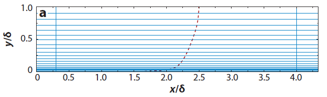
In the case of Detached Eddy Simulations (DES), there are two regions in a computational domain that are treated in RANS-like and LES-like manners. The original Spalart-Allmaras DES model (DES97) formulation is based on the assumption that the wall-parallel grid spacing near the wall is in excess of the boundary-layer thickness \(\delta\) by a good margin so that the entire boundary layer can be handled by RANS [1].
Fig. 1 Natural DES grid in a boundary layer. Dotted line means velocity profile. \(\delta\) is the boundary-layer thickness [1].
Settings of DESModelRegions
In OpenFOAM, we can visually check these regions using the DESModelRegions function objects. It is also available in iconCFD.
DES (Detached Eddy Simulation) turbulence model is pioneered in 1997 by Spalart et al. based on the Spalart-Allmaras RANS model [1]. It is referred to as DES97 model in the CFD (Computational Fluid Dynamics) community and several improved versions (DDES and IDDES) have been developed so far that have continually widened the areas of application. They have been implemented in both commercial and open-source CFD softwares and used on a regular basis in both industry and academia.
In this blog post, I will try to describe in detail DES97 model that serves as a base for the subsequent models:
The motivation and aim of DES models is to decrease the computational cost of massively separated turbulent flows compared to LES (Large Eddy Simulation). The reduction in the cost is achieved by modeling the boundary layers using unsteady RANS (Reynolds-Averaged Navier-Stokes) model [2].
Detached-Eddy Simulation (DES) is a hybrid technique first proposed by Spalart et al. (1997) for prediction of turbulent flows at high Reynolds numbers (see also Spalart 2000). Development of the technique was motivated by estimates which indicate that the computational costs of applying Large-Eddy Simulation (LES) to complete configurations such as an airplane, submarine, or road vehicle are prohibitive. The high cost of LES when applied to complete configurations at high Reynolds numbers arises because of the resolution required in the boundary layers, an issue that remains even with fully successful wall-layer modeling.
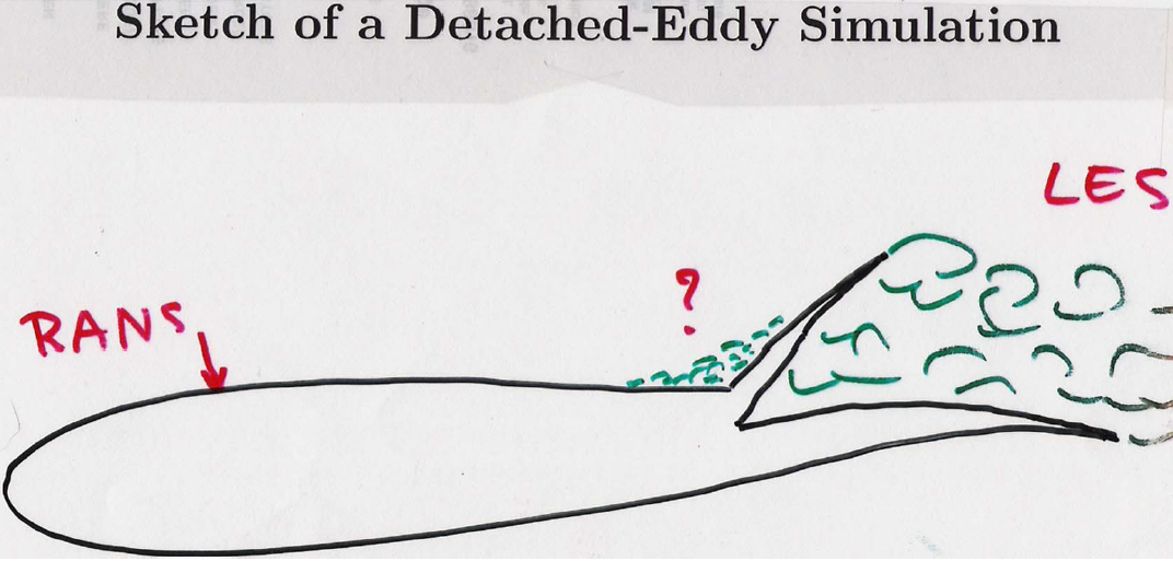
In Detached-Eddy Simulation (DES), the aim is to combine the most favorable aspects of the two techniques, i.e., application of RANS models for predicting the attached boundary layers and LES for resolution of time-dependent, three-dimensional large eddies. The cost scaling of the method is then favorable since LES is not applied to resolution of the relatively smaller-structures that populate the boundary layer.
Fig. 1 Sketch of a Detached-Eddy Simulation [7]The DES97 model accomplishes the switching between RANS and LES modes by changing the length scale as will be described later in this post.
The model is available in OpenFOAM. I will detail its implementations in various OpenFOAM versions.
Mathematical Expression
\begin{align}
&\;\frac{\partial (\rho \tilde{\nu})}{\partial t} + \frac{\partial (\rho u_j \tilde{\nu})}{\partial x_j} \\
-&\;\frac{1}{\sigma} \left[ \frac{\partial}{\partial x_j} \left( \rho \left( \tilde{\nu} + \nu \right) \frac{\partial \tilde{\nu}}{\partial x_j} \right) + C_{b2} \rho \frac{\partial \tilde{\nu}}{\partial x_i} \frac{\partial \tilde{\nu}}{\partial x_i} \right] \tag{1} \label{eq:sa4} \\
=&\;C_{b1} \rho \tilde{S} \tilde{\nu}\;-\;C_{w1} \rho f_{w} \left( \frac{\tilde{\nu}}{\tilde{d}} \right)^2
\end{align}
In the case of incompressible fluid flow, the density \(\rho = 1\) in Eq. \eqref{eq:sa4}. The third term in the l.h.s. of Eq. \eqref{eq:sa4} is the diffusion term. In the r.h.s, the terms starting from the left represent the production and destruction terms for the eddy viscosity \(\tilde{\nu}\). The destruction term is changed from the Spalart-Allmaras RANS model by replacing the distance to the wall \(d\) with a new length scale \(\tilde{d}\) [2]
\begin{equation}
\tilde{d} = {\rm min} \left( l_{RANS}, l_{LES} \right) = {\rm min} \left( d, C_{DES}\Delta \right) \tag{2} \label{eq:dTilda}
\end{equation}
where \(\Delta\) is the chosen measure of grid spacing and \(C_{DES}\) is a calibration constant and its default value is 0.65.
When balanced with the production term, this term adjusts the eddy viscosity to scale with the local deformation rate \(S\) and \(d\): \(\tilde{\nu} \propto Sd^2\). Subgrid-scale (SGS) eddy viscosities scale with \(S\) and the grid spacing \(\Delta\), i.e., \(\nu_{SGS} \propto S\Delta^2\). A subgrid-scale model within the S-A formulation can then be obtained by replacing \(d\) with a length scale \(\Delta\) directly proportional to the grid spacing.
The \(f_{t2}\) laminar suppression term is included in com versions (v1606+ – v1812) as against v4. The subscript \(t\) stands for “trip”. The production term is multiplied by \(1-f_{t2}\) so that \(\tilde{\nu} = 0\) is a stable solution when solving a transitional flow where both laminar and turbulent regions exist in one computational domain. The destruction term is also altered in accordance with the change in the production term in order to balance the energy budget near the wall [3]. For fully turbulent flows at high Reynolds numbers, the \(f_{t2}\) term takes small values and makes essentially no difference between the above two equations.
In addition to this difference, the low-Reynolds number correction option [4] is available only in com versions (v1606+ – v1812):
If the low-Re number correction option is deactivated (lowReCorrection false;) and the value of \(C_{t3}\) is set to 0 in v1606+ – v1812, the same calculation can be done as v4.
Low-Reynolds Number Term Correction \(\Psi\) Function
The low-Reynolds number terms in the S-A RANS model were designed to account for wall proximity, “measured” by the ratio of the eddy and molecular viscosities \(\nu_t/\nu\) (an expedient to avoid using the friction velocity). Most RANS models have similar terms, also based on various turbulent Reynolds numbers. However, in the LES mode of DES, the subgrid eddy viscosity (normalized by the molecular viscosity) decreases with grid refinement and decrease of the flow Reynolds number. At some point, standard DES will mis-interpret the situation as “wall proximity” and lower the eddy viscosity excessively, relative to the ambient velocity and length scales, through the \(f_v\) and \(f_t\) functions of the S-A model. Although this deficiency shows up only at relatively low Reynolds numbers and/or with very fine grids, it is still desirable to eliminate it, and to do so without zonal instructions from the user.
The DES97 model is based on the assumption that the wall-parallel grid spacing near the wall \(\Delta_{||}\) is in excess of the boundary layer thickness \(\delta\) by a good margin so that the entire boundary layer is handled by RANS model. As we can see from Eq. \eqref{eq:dTilda}, the new length scale of DES97 model \(\tilde{d}\) depends only on the geometric features of computational mesh and not on the computed flow fields at all.
If we choose the following measure of grid spacing that is maxDeltaxyz option in OpenFOAM
\begin{equation}
\Delta \equiv {\rm max} \left( \Delta x, \Delta y, \Delta z \right), \tag{6} \label{eq:delta}
\end{equation}
the wall-parallel grid spacing \(\Delta_{||}\) should meet the following inequality to satisfy the above mesh requirement
\begin{equation}
\Delta_{||} \approx \Delta \geq \frac{d}{C_{DES}} \geq \frac{\delta}{C_{DES}}, \tag{7} \label{eq:deltaInequality}
\end{equation}
where we assume that \(y\) is the wall normal direction and \(\Delta_{||} \approx \Delta_x \approx \Delta_z\).
There are several problems that DES97 model suffers from.
Grey area
Modeled-Stress Depletion (MSD)
Delayed DES and Zonal DES are the solutions to MSD.
Grid-induced Separation (GIS)
MSD is the root cause of GIS.
Laminar Suppression Term ft2
In the excellent Turbulence Modeling Resource page [5] of NASA Langley Research Center, the various deformations of the Spalart-Allmaras turbulence (RANS) model are clearly documented.
According to the naming method, the “Standard” Spalart-Allmaras One-Equation Model (SA) is implemented in OpenFOAM v1606+ – v1812 and the Spalart-Allmaras One-Equation Model without \(f_{t2}\) Term (SA-noft2) is implemented in v4.
Spalart-Allmaras One-Equation Model without \(f_{t2}\) Term (SA-noft2) Many implementations of Spalart-Allmaras ignore the \(f_{t2}\) term, which was a numerical fix in the original model in order to make zero a stable solution to the equation with a small basin of attraction (thus slightly delaying transition so that the trip term could be activated appropriately). It is argued that if the trip is not used, then \(f_{t2}\) is not necessary. The equations are the same as for the “standard” version (SA), except that the term \(f_{t2}\) does not appear at all (i.e., ct3=0 instead of 1.2).
The fvOptions functionality in OpenFOAM is flexible framework to add various source terms to the governing equations without the need to rewrite the original source code. The available options in the latest versions of OpenFOAM (v4.0 and v1606+) are listed below.
My explanations are available for the options shown in red.
to add a porosity momentum source term in all cells or user-specified cellZone or cellSet (available porosity models: fixedCoeff, powerLaw and DarcyForchheimer)
to emulate a flow blockage effect due to the neighbour region by adding a inter-regional porosity momentum source in the overlapped volume with the neighbour region
to simulate the fluid flow in a domain that is in 6-DoF solid-body motion without dynamic mesh by adding the fictitious force terms, e.g., the Coriolis, Centrifugal and Euler forces in a non-inertial reference frame
to damp the acoustic waves before they reach the boundaries by adding a momentum source term in a buffer region so that the solution will not be contaminated by the reflected waves from the boundaries
When specifying a source term using fvOptions in OpenFOAM, we can select the selectionMode (how to set the source region) from the following four options:
points
cellSet
cellZone
all
The meanings of these options are described in this post.
The boundary conditions of HbyA are now constrained by the new “constrainHbyA” function which applies the velocity boundary values for patches for which the velocity cannot be modified by assignment and pressure extrapolation is not specified via the new “fixedFluxExtrapolatedPressureFvPatchScalarField”.
dotInterpolate interpolates the field and “dots” the resulting face-values with the vector field provided which removes the need to create a temporary field for the interpolate. This reduces the peak storage of OpenFOAM caused by the divergence of the gradient of vector fields, improves memory management and under some conditions decreases run-time.
This development is based on a patch contributed by Paul Edwards, Intel.
In the case of compressible flow, the following relation \eqref{eq:1} holds for the velocity on the face:
\begin{equation}
\rho \boldsymbol{U}_f \cdot \boldsymbol{S}_f = \left(\frac{\rho \boldsymbol{H}}{A_p}\right)_f \cdot \boldsymbol{S}_f\;-\;\left(\frac{\rho}{A_p}\right)_f (\nabla p)_f \cdot \boldsymbol{S}_f. \tag{1} \label{eq:1}
\end{equation}
Thus
\begin{equation}
(\nabla p)_f \cdot \boldsymbol{n}_f = \frac{1}{|\boldsymbol{S}_f|\left(\frac{\rho}{A_p}\right)_f} \left(\left(\frac{\rho \boldsymbol{H}}{A_p}\right)_f \cdot \boldsymbol{S}_f\;-\;\rho \boldsymbol{U}_f \cdot \boldsymbol{S}_f \right). \tag{2} \label{eq:2}
\end{equation}
The fixedFluxPressure boundary condition calculates the boundary normal gradient of the pressure field using the Eq. \eqref{eq:2} so that the boundary fluxes satisfy the Eq. \eqref{eq:1}.
Many function objects and sampling utilities are able to export field data. In earlier versions of OpenFOAM, the surface data file contained both the geometry and field data. For transient data output, this leads to the geometry being written multiple times, even if it remains static. In this release, surfaceWriter with Ensight format has been re-written to allow the geometry to be written only once. To enable this feature, a new option collateTimes has been added.
system/controlDict file
C++
1
2
3
4
5
6
7
8
9
10
11
12
13
14
15
16
17
18
19
20
21
22
23
24
25
26
27
28
29
30
31
32
33
34
35
36
37
functions
{
section
{
type surfaces;
outputControl timeStep;
outputInterval20;
surfaceFormat ensight;
interpolationScheme cell;
fields
(
T
);
surfaces
(
plane1
{
type plane;
basePoint(000);
normalVector(001);
interpolate false;
}
);
formatOptions
{
ensight
{
// Write single mesh file
// (only for static surfaces)
collateTimes true;
}
}
}
}
The structures of the postProcessing directory are different with and without the collateTimes option as shown below.
When specifying a source term using fvOptions in OpenFOAM, we can select the selectionMode (how to set the source region) from the following four options:
points
cellSet
cellZone
all
These options are defined in the cellSetOption class along with the other common parameters among the fvOptions such as timeStart and duration. Let’s check out the meaning of each option along with its source code.
selectionMode 1: points
In this case, we specify some points as shown in the following example. The source region consists of the individual cells that contain the specified points.
Example of description
1
2
3
4
5
6
selectionMode points;
points
(
(-0.010.010)
(0.03-0.0150)
);
Source code
92
93
94
95
96
97
98
99
100
101
102
103
104
105
106
107
108
109
110
111
112
113
114
115
116
117
118
119
120
121
122
123
voidFoam::fv::cellSetOption::setCellSet()
{
switch(selectionMode_)
{
casesmPoints:
{
Info<<indent<<"- selecting cells using points"<<endl;
<<"Unable to find owner cell for point "<<points_[i]
<<endl;
}
}
cells_=selectedCells.toc();
break;
}
selectionMode 2: cellSet
In this case, we preliminarily create a cellSet corresponding to the source region using OpenFOAM’s utilities such as setSet and specify the created cellSet name.
Example of description
1
2
selectionMode cellSet;
cellSet cSet1;
Source code
124
125
126
127
128
129
130
131
132
133
casesmCellSet:
{
Info<<indent
<<"- selecting cells using cellSet "<<cellSetName_<<endl;
cellSet selectedCells(mesh_,cellSetName_);
cells_=selectedCells.toc();
break;
}
selectionMode 3: cellZone
In this case, we preliminarily create a cellZone corresponding to the source region using OpenFOAM’s utilities such as setSet and specify the created cellZone name.
Example of description
1
2
selectionMode cellZone;
cellZone cZone1;
Source code
134
135
136
137
138
139
140
141
142
143
144
145
146
147
148
149
150
casesmCellZone:
{
Info<<indent
<<"- selecting cells using cellZone "<<cellSetName_<<endl;
selectionMode: [Required] Domain the source is applied (all/cellSet/cellZone/points)
The parameter name fields has been changed from fieldNames in the latest version as described in this page.
The meanVelocityForce fvOptions calculates a momentum source so that the volume averaged velocity \eqref{eq:magUbarAve} in the whole computational domain (all) or a part of domain specified using cellSet or cellZone reaches the desired mean velocity Ubar.
\begin{align}
\frac{\sum_{i}^{} \left(\frac{\bar{\boldsymbol{u}}}{|\bar{\boldsymbol{u}}|} \cdot \boldsymbol{u}_i \right)V_i}{\sum_{i}^{} V_i}, \tag{1} \label{eq:magUbarAve}
\end{align}
where the summation is over the cells that belong to the user-specified domain, \(\bar{\boldsymbol{u}}\) is Ubar, \(\boldsymbol{u}_i\) is the velocity in the i-th cell and \(V_i\) is the volume of the i-th cell.
patchMeanVelocityForce
The patchMeanVelocityForce fvOptions is also available to specify the desired mean velocity on a patch instead of the volumetric average \eqref{eq:magUbarAve}.
In what follows, we will take a closer look at each of three highlighted lines when the meanVelocityForce fvOptions is used. The source files of this class are in src/fvOptions/sources/derived/meanVelocityForce.
l. 11
The addSup function is called from l.11 in UEqn.H when discretizing the momentum equation and source term Su is added to the equation.
The constrain function is called from l.17 in UEqn.H. The if loop is true in the first iteration and else loop is executed for the other iterations to initialize and update the volScalarField defined as the reciprocal of the diagonal coefficients.
constrain function in meanVelocityForce.C
C++
229
230
231
232
233
234
235
236
237
238
239
240
241
242
243
244
245
246
247
248
249
250
251
252
253
254
255
256
257
258
259
260
voidFoam::fv::meanVelocityForce::constrain
(
fvMatrix<vector>&eqn,
constlabel
)
{
if(rAPtr_.empty())
{
rAPtr_.reset
(
newvolScalarField
(
IOobject
(
name_+":rA",
mesh_.time().timeName(),
mesh_,
IOobject::NO_READ,
IOobject::NO_WRITE
),
1.0/eqn.A()
)
);
}
else
{
rAPtr_()=1.0/eqn.A();
}
gradP0_+=dGradP_;
dGradP_=0.0;
}
l. 23
As the average velocity magUbarAve \eqref{eq:magUbarAve} reaches a user-specified value Ubar, the pressure gradient increment dGradP_ needed to adjust the average velocity converges to 0.