It is computationally expensive to resolve the wide range of time and length scales observed in turbulent flows. We now consider decomposing a flow property \(f\), such as velocity and pressure, into a mean component \(\overline{f}\) and a fluctuating component \(f’\).
\begin{equation}
f(\boldsymbol{x}, t) = \overline{f}(\boldsymbol{x}, t) + f'(\boldsymbol{x}, t), \tag{1} \label{eq:decomposition}
\end{equation}
where \(\boldsymbol{x}\) is the position vector and \(t\) is time.
The Reynolds-averaged Navier-Stokes (RANS) turbulence models aim to solve the mean flow \(\overline{f}\) that changes more slowly in time and space than the original variable \(f\). The governing equations of the mean component will be derived later.
There are many averaging operations defined in mathematics but the RANS models use the Reynolds average. It is briefly described in the newly published textbook by Kajishima and Taira [1].
For the discussion in this chapter, let us redefine the averaging operation such that it satisfies
\begin{equation}
\overline{f’} = 0,\;\;\overline{f’ \overline{f}} = 0,\;\;\overline{\overline{f}} = \overline{f}. \tag{7.2} \label{eq:reave}
\end{equation}
These relations in Eq. \eqref{eq:reave} are referred to as the Reynolds-averaging laws. The ensemble average that satisfies these laws is called the Reynolds average. This conceptual averaging operation conveniently removes fluctuating components from the flow field variables without explicitly defining the spatial length scale used in the averaging operation.
The ensemble average that appears in the above definition is defined as (and usually denoted as \(\langle f \rangle\))
\begin{equation}
\langle f \rangle(\boldsymbol{x}, t) \equiv \lim_{N \to \infty}\frac{1}{N}\sum_{i=1}^{N}f_{i}(\boldsymbol{x}, t), \tag{2} \label{eq:ensembleAve}
\end{equation}
where \(f_i\) are the samples of \(f\) and \(N\) is the number of samples. In other words, it is the average of the instantaneous values of the property at a given point in space \(\boldsymbol{x}\) and time \(t\) over a large number of repeated identical experiments. In general, this ensemble average varies with space and time (time-dependent).
For the stationary random processes, we can define the time average \(f_T\):
\begin{equation}
f_{T}(\boldsymbol{x}) \equiv \frac{1}{T} \int_{0}^{T} f(\boldsymbol{x}, t) dt, \tag{3} \label{eq:timeAve}
\end{equation}
where \(T\) is the integration time. In the case of stationary random processes, the time averages equal the ensemble averages as stated in [3]:
if the signal is stationary, the time average defined by equation \eqref{eq:timeAve} is an unbiased estimator of the true average \(\langle f \rangle\). Moreover, the estimator converges to \(\langle f \rangle\) as the time becomes infinite; i.e., for stationary random processes
\begin{equation}
\langle f \rangle(\boldsymbol{x}) = \lim_{T \to \infty} \frac{1}{T} \int_{0}^{T} f(\boldsymbol{x}, t) dt, \tag{8.28} \label{eq:aveRelation}
\end{equation}
Thus the time and ensemble averages are equivalent in the limit as \(T \to \infty\), but only for a stationary random process.
Interested readers might want to search by the keyword ”ergodic hypothesis” on the relation between the ensemble and time averages.
RANS Equations
To Be Updated
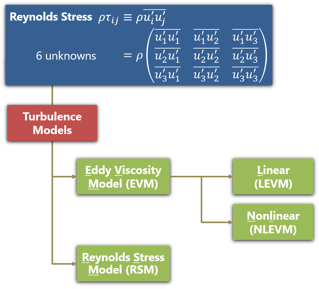
Closure Problem – Reynolds Stress
The linear eddy viscosity models (LEVM) assume the linear stress-strain relationship and employ the eddy-viscosity concept (Boussinesq approximation) introduced by Joseph Valentin Boussinesq
\begin{equation}
-\rho\overline{u_i u_j} = \mu_t \left(\frac{\partial \overline{U}_i}{\partial x_j} + \frac{\partial \overline{U}_j}{\partial x_i} \right) -\frac{2}{3}\delta_{ij}\rho k. \tag{4} \label{eq:BoussinesqApprox}
\end{equation}
[1] T. Kajishima and K. Taira, Computational Fluid Dynamics: Incompressible Turbulent Flows. Springer, 2016.
[2] H. K. Versteeg and W. Malalasekera, An introduction to Computational Fluid Dynamics: The Finite Volume Method. Person Prentice Hall, 1995.
[3] W. K. George, Lectures in Turbulence for the 21st Century.
The DES length scale \(\tilde{d}\) is modified compared to that of DES97 model to prevent a premature switch of DES to LES mode within boundary layers. This incursion can be a cause of modeled-stress depletion (MSD) issue that the DES97 formulation suffers from.
Two functions \(r_d\) and \(f_d\) are introduced in new definition \eqref{eq:dTilda} and it now depends not only on the grid but also the time-dependent eddy-viscosity field as Eq. \eqref{eq:rd} shows. The new length scale \eqref{eq:dTilda} detects the boundary layer and delays the switch to LES mode until outside of it. For this reason, the method was named delayed DES.
\begin{equation}
r_d \equiv \frac{\nu_t + \nu}{\sqrt{U_{i,j}U_{i,j}}\kappa^2 d^2} \tag{1} \label{eq:rd}
\end{equation}
where \(\nu_{t}\) is the kinematic eddy viscosity, \(\nu\) the molecular viscosity, \(U_{i,j}\) the velocity gradients, \(\kappa\) the Kármán constant and \(d\) the distance to the wall.
The quantity \(r_{d}\) is used in the shielding function \(f_{d}\):
\begin{equation}
f_d \equiv 1 – {\rm tanh} \left[ \left( 8r_d \right)^3 \right] \tag{2} \label{eq:fd}
\end{equation}
which is designed to be 1 in the LES region, where \(r_{d}\ \ll 1\), and 0 elsewhere.
\begin{equation}
\tilde{d} \equiv d \; – f_d {\rm max}(0, d \; – \; C_{DES}\Delta) \tag{3} \label{eq:dTilda}
\end{equation}
References
[1] P. R. Spalart, S. Deck, M. L. Shur, K. D. Squires, M. Kh. Strelets and A. Travin, A new version of detached-eddy simulation, resistant to ambiguous grid densities. Theoretical and Computational Fluid Dynamics 20(3), 181-195, 2006.
Description
Apply a simplified boundary-layer model to the velocity and turbulence fields based on the 1/7th power-law.
The uniform boundary-layer thickness is either provided via the -ybl option or calculated as the average of the distance to the wall scaled with the thickness coefficient supplied via the option -Cbl. If both options are provided -ybl is used.
The velocity profile is initialized based on the 1/7th power law turbulent velocity profile:
\begin{equation}
\boldsymbol{u} = \boldsymbol{U} \left( \frac{y_w}{\delta} \right)^{\frac{1}{7}}, \tag{1}
\end{equation}
where \(\boldsymbol{U}\) is the main flow velocity, \(y_w\) is the distance to the wall and \(\delta\) is the boundary-layer thickness.
applyBoundaryLayer.C
C++
101
102
103
104
105
106
107
108
109
110
111
112
113
114
115
116
117
118
119
120
121
122
// Modify velocity by applying a 1/7th power law boundary-layer
// u/U0 = (y/ybl)^(1/7)
// assumes U0 is the same as the current cell velocity
This report documents the results of a study to address the long range, strategic planning required by NASA’s Revolutionary Computational Aerosciences (RCA) program in the area of computational fluid dynamics (CFD), including future software and hardware requirements for High Performance Computing (HPC). Specifically, the “Vision 2030” CFD study is to provide a knowledge-based forecast of the future computational capabilities required for turbulent, transitional, and reacting flow simulations across a broad Mach number regime, and to lay the foundation for the development of a future framework and/or environment where physics-based, accurate predictions of complex turbulent flows, including flow separation, can be accomplished routinely and efficiently in cooperation with other physics-based simulations to enable multi-physics analysis and design. Specific technical requirements from the aerospace industrial and scientific communities were obtained to determine critical capability gaps, anticipated technical challenges, and impediments to achieving the target CFD capability in 2030. A preliminary development plan and roadmap were created to help focus investments in technology development to help achieve the CFD vision in 2030.
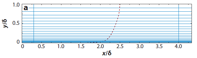
In the case of Detached Eddy Simulations (DES), there are two regions in a computational domain that are treated in RANS-like and LES-like manners. The original Spalart-Allmaras DES model (DES97) formulation is based on the assumption that the wall-parallel grid spacing near the wall is in excess of the boundary-layer thickness \(\delta\) by a good margin so that the entire boundary layer can be handled by RANS [1].
Fig. 1 Natural DES grid in a boundary layer. Dotted line means velocity profile. \(\delta\) is the boundary-layer thickness [1].
Settings of DESModelRegions
In OpenFOAM, we can visually check these regions using the DESModelRegions function objects. It is also available in iconCFD.
DES (Detached Eddy Simulation) turbulence model is pioneered in 1997 by Spalart et al. based on the Spalart-Allmaras RANS model [1]. It is referred to as DES97 model in the CFD (Computational Fluid Dynamics) community and several improved versions (DDES and IDDES) have been developed so far that have continually widened the areas of application. They have been implemented in both commercial and open-source CFD softwares and used on a regular basis in both industry and academia.
In this blog post, I will try to describe in detail DES97 model that serves as a base for the subsequent models:
The motivation and aim of DES models is to decrease the computational cost of massively separated turbulent flows compared to LES (Large Eddy Simulation). The reduction in the cost is achieved by modeling the boundary layers using unsteady RANS (Reynolds-Averaged Navier-Stokes) model [2].
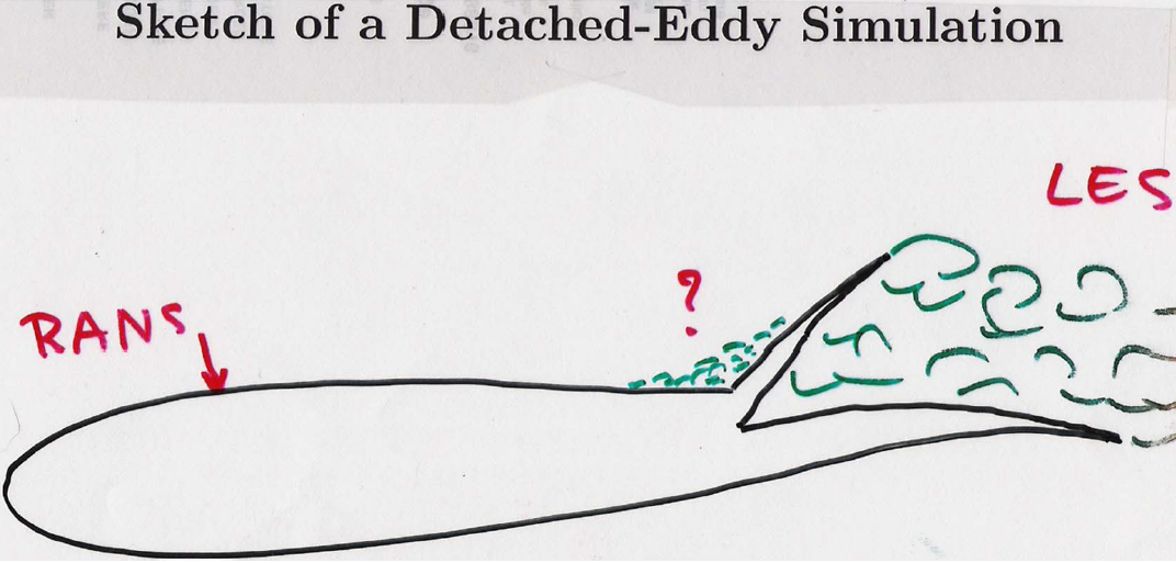
Detached-Eddy Simulation (DES) is a hybrid technique first proposed by Spalart et al. (1997) for prediction of turbulent flows at high Reynolds numbers (see also Spalart 2000). Development of the technique was motivated by estimates which indicate that the computational costs of applying Large-Eddy Simulation (LES) to complete configurations such as an airplane, submarine, or road vehicle are prohibitive. The high cost of LES when applied to complete configurations at high Reynolds numbers arises because of the resolution required in the boundary layers, an issue that remains even with fully successful wall-layer modeling.
In Detached-Eddy Simulation (DES), the aim is to combine the most favorable aspects of the two techniques, i.e., application of RANS models for predicting the attached boundary layers and LES for resolution of time-dependent, three-dimensional large eddies. The cost scaling of the method is then favorable since LES is not applied to resolution of the relatively smaller-structures that populate the boundary layer.
Fig. 1 Sketch of a Detached-Eddy Simulation [7]The DES97 model accomplishes the switching between RANS and LES modes by changing the length scale as will be described later in this post.
The model is available in OpenFOAM. I will detail its implementations in various OpenFOAM versions.
Mathematical Expression
\begin{align}
&\;\frac{\partial (\rho \tilde{\nu})}{\partial t} + \frac{\partial (\rho u_j \tilde{\nu})}{\partial x_j} \\
-&\;\frac{1}{\sigma} \left[ \frac{\partial}{\partial x_j} \left( \rho \left( \tilde{\nu} + \nu \right) \frac{\partial \tilde{\nu}}{\partial x_j} \right) + C_{b2} \rho \frac{\partial \tilde{\nu}}{\partial x_i} \frac{\partial \tilde{\nu}}{\partial x_i} \right] \tag{1} \label{eq:sa4} \\
=&\;C_{b1} \rho \tilde{S} \tilde{\nu}\;-\;C_{w1} \rho f_{w} \left( \frac{\tilde{\nu}}{\tilde{d}} \right)^2
\end{align}
In the case of incompressible fluid flow, the density \(\rho = 1\) in Eq. \eqref{eq:sa4}. The third term in the l.h.s. of Eq. \eqref{eq:sa4} is the diffusion term. In the r.h.s, the terms starting from the left represent the production and destruction terms for the eddy viscosity \(\tilde{\nu}\). The destruction term is changed from the Spalart-Allmaras RANS model by replacing the distance to the wall \(d\) with a new length scale \(\tilde{d}\) [2]
\begin{equation}
\tilde{d} = {\rm min} \left( l_{RANS}, l_{LES} \right) = {\rm min} \left( d, C_{DES}\Delta \right) \tag{2} \label{eq:dTilda}
\end{equation}
where \(\Delta\) is the chosen measure of grid spacing and \(C_{DES}\) is a calibration constant and its default value is 0.65.
When balanced with the production term, this term adjusts the eddy viscosity to scale with the local deformation rate \(S\) and \(d\): \(\tilde{\nu} \propto Sd^2\). Subgrid-scale (SGS) eddy viscosities scale with \(S\) and the grid spacing \(\Delta\), i.e., \(\nu_{SGS} \propto S\Delta^2\). A subgrid-scale model within the S-A formulation can then be obtained by replacing \(d\) with a length scale \(\Delta\) directly proportional to the grid spacing.
The \(f_{t2}\) laminar suppression term is included in com versions (v1606+ – v1812) as against v4. The subscript \(t\) stands for “trip”. The production term is multiplied by \(1-f_{t2}\) so that \(\tilde{\nu} = 0\) is a stable solution when solving a transitional flow where both laminar and turbulent regions exist in one computational domain. The destruction term is also altered in accordance with the change in the production term in order to balance the energy budget near the wall [3]. For fully turbulent flows at high Reynolds numbers, the \(f_{t2}\) term takes small values and makes essentially no difference between the above two equations.
In addition to this difference, the low-Reynolds number correction option [4] is available only in com versions (v1606+ – v1812):
If the low-Re number correction option is deactivated (lowReCorrection false;) and the value of \(C_{t3}\) is set to 0 in v1606+ – v1812, the same calculation can be done as v4.
Low-Reynolds Number Term Correction \(\Psi\) Function
The low-Reynolds number terms in the S-A RANS model were designed to account for wall proximity, “measured” by the ratio of the eddy and molecular viscosities \(\nu_t/\nu\) (an expedient to avoid using the friction velocity). Most RANS models have similar terms, also based on various turbulent Reynolds numbers. However, in the LES mode of DES, the subgrid eddy viscosity (normalized by the molecular viscosity) decreases with grid refinement and decrease of the flow Reynolds number. At some point, standard DES will mis-interpret the situation as “wall proximity” and lower the eddy viscosity excessively, relative to the ambient velocity and length scales, through the \(f_v\) and \(f_t\) functions of the S-A model. Although this deficiency shows up only at relatively low Reynolds numbers and/or with very fine grids, it is still desirable to eliminate it, and to do so without zonal instructions from the user.
The DES97 model is based on the assumption that the wall-parallel grid spacing near the wall \(\Delta_{||}\) is in excess of the boundary layer thickness \(\delta\) by a good margin so that the entire boundary layer is handled by RANS model. As we can see from Eq. \eqref{eq:dTilda}, the new length scale of DES97 model \(\tilde{d}\) depends only on the geometric features of computational mesh and not on the computed flow fields at all.
If we choose the following measure of grid spacing that is maxDeltaxyz option in OpenFOAM
\begin{equation}
\Delta \equiv {\rm max} \left( \Delta x, \Delta y, \Delta z \right), \tag{6} \label{eq:delta}
\end{equation}
the wall-parallel grid spacing \(\Delta_{||}\) should meet the following inequality to satisfy the above mesh requirement
\begin{equation}
\Delta_{||} \approx \Delta \geq \frac{d}{C_{DES}} \geq \frac{\delta}{C_{DES}}, \tag{7} \label{eq:deltaInequality}
\end{equation}
where we assume that \(y\) is the wall normal direction and \(\Delta_{||} \approx \Delta_x \approx \Delta_z\).
There are several problems that DES97 model suffers from.
Grey area
Modeled-Stress Depletion (MSD)
Delayed DES and Zonal DES are the solutions to MSD.
Grid-induced Separation (GIS)
MSD is the root cause of GIS.
Laminar Suppression Term ft2
In the excellent Turbulence Modeling Resource page [5] of NASA Langley Research Center, the various deformations of the Spalart-Allmaras turbulence (RANS) model are clearly documented.
According to the naming method, the “Standard” Spalart-Allmaras One-Equation Model (SA) is implemented in OpenFOAM v1606+ – v1812 and the Spalart-Allmaras One-Equation Model without \(f_{t2}\) Term (SA-noft2) is implemented in v4.
Spalart-Allmaras One-Equation Model without \(f_{t2}\) Term (SA-noft2) Many implementations of Spalart-Allmaras ignore the \(f_{t2}\) term, which was a numerical fix in the original model in order to make zero a stable solution to the equation with a small basin of attraction (thus slightly delaying transition so that the trip term could be activated appropriately). It is argued that if the trip is not used, then \(f_{t2}\) is not necessary. The equations are the same as for the “standard” version (SA), except that the term \(f_{t2}\) does not appear at all (i.e., ct3=0 instead of 1.2).