Tensor Operations in OpenFOAM

Last Updated: May 5, 2019

The gradient of the velocity field is a strain-rate tensor field, that is, a second rank tensor field. It appears in the diffusion term of the Navier-Stokes equation.

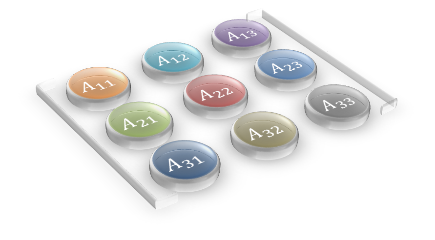
A second rank tensor has nine components and can be expressed as a 3×3 matrix as shown in the above image.

In this blog post, I will pick out some typical tensor operations and give brief explanations of them with some usage examples in OpenFOAM.

Keywords
strain rate tensor, vorticity tensor, Q-criterion, Hodge dual

Gradient of a Vector Field | fvc::grad(u)

The gradient of a velocity vector \(\boldsymbol{u}\) returns a velocity gradient tensor (second rank tensor).
\begin{eqnarray}
\nabla \boldsymbol{u} &\equiv& \partial_{i} u_j \\
&=& \left(
\begin{matrix}
\partial u_1/\partial x_1 & \partial u_2/\partial x_1 & \partial u_3/\partial x_1 \\
\partial u_1/\partial x_2 & \partial u_2/\partial x_2 & \partial u_3/\partial x_2 \\
\partial u_1/\partial x_3 & \partial u_2/\partial x_3 & \partial u_3/\partial x_3
\end{matrix} \right)
\end{eqnarray}

Symmetric Part of a Second Rank Tensor | symm(T)

\begin{eqnarray}
{\rm symm}(\boldsymbol{T}) &\equiv& \frac{1}{2} (\boldsymbol{T} + \boldsymbol{T}^T) \\
&=& \frac{1}{2} \left(
\begin{matrix}
2T_{11} & T_{12} + T_{21} & T_{13} + T_{31} \\
T_{21} + T_{12} & 2T_{22} & T_{23} + T_{32} \\
T_{31} + T_{13} & T_{32} + T_{23} & 2T_{33}
\end{matrix} \right)
\end{eqnarray}

Twice the Symmetric Part of a Second Rank Tensor | twoSymm(T)

\begin{eqnarray}
{\rm twoSymm}(\boldsymbol{T}) &\equiv& \boldsymbol{T} + \boldsymbol{T}^T \\
&=& \left(
\begin{matrix}
2T_{11} & T_{12} + T_{21} & T_{13} + T_{31} \\
T_{21} + T_{12} & 2T_{22} & T_{23} + T_{32} \\
T_{31} + T_{13} & T_{32} + T_{23} & 2T_{33}
\end{matrix} \right)
\end{eqnarray}

Skew-symmetric Part of a Second Rank Tensor | skew(T)

\begin{eqnarray}
{\rm skew}(\boldsymbol{T}) &\equiv& \frac{1}{2} (\boldsymbol{T} – \boldsymbol{T}^T) \\
&=& \frac{1}{2} \left(
\begin{matrix}
0 & T_{12} – T_{21} & T_{13} – T_{31} \\
T_{21} – T_{12} & 0 & T_{23} – T_{32} \\
T_{31} – T_{13} & T_{32} – T_{23} & 0
\end{matrix} \right)
\end{eqnarray}

The symm and skew operations of the velocity gradient tensor field frequently appear in the source code. The following is a typical example.

In the above code, the symmetric and antisymmetric parts of the velocity gradient tensor \(\partial u_j/\partial x_i\) are defined as follows:
\begin{eqnarray}
S_{ij} &=& \frac{1}{2} \left( \frac{\partial u_j}{\partial x_i} + \frac{\partial u_i}{\partial x_j} \right), \\
\Omega_{ij} &=& \frac{1}{2} \left( \frac{\partial u_j}{\partial x_i} – \frac{\partial u_i}{\partial x_j} \right),
\end{eqnarray}
where \(S_{ij}\) is the strain rate tensor and \(-\Omega_{ij}\) is the vorticity (spin) tensor.

Hodge Dual | *T

\begin{equation}
*T = \left( T_{23},\;-T_{13},\;T_{12} \right)
\end{equation}

The vorticity vector \(\boldsymbol{\omega}\) is calculated as the Hodge dual of the skew-symmetric part of the velocity gradient tensor.
\begin{eqnarray}
\boldsymbol{\omega} &=& 2 \times \left( * \Omega_{ij} \right) \\
&=& 2 \times \left( \Omega_{23},\;-\Omega_{13},\;\Omega_{12} \right) \\
&=& \left( \frac{\partial u_3}{\partial x_2}-\frac{\partial u_2}{\partial x_3},\;\frac{\partial u_1}{\partial x_3}-\frac{\partial u_3}{\partial x_1},\;\frac{\partial u_2}{\partial x_1}-\frac{\partial u_1}{\partial x_2} \right)
\end{eqnarray}

The operator * in front of the skew is the Hodge dual operator.

Inner Product of Two Second Rank Tensors | T & S

\begin{equation}
P_{ij} = T_{ik} S_{kj}
\end{equation}

Double Inner Product of Two Second Rank Tensors | T && S

\begin{align}
s = T_{ij}S_{ij} &= T_{11}S_{11} + T_{12}S_{12} + T_{13}S_{13} \\
&+ T_{21}S_{21} + T_{22}S_{22} + T_{23}S_{23} \\
&+ T_{31}S_{31} + T_{32}S_{32} + T_{33}S_{33}
\end{align}

Trace of a Second Rank Tensor | tr(T)

\begin{equation}
{\rm tr}(\boldsymbol{T}) \equiv T_{11} + T_{22} + T_{33} = \boldsymbol{T} {\rm \&}{\rm \&} \boldsymbol{I}
\end{equation}

The Q-criterion can be used to identify vortex cores:
\begin{align}
Q &= \frac{1}{2} \left[ (\nabla \cdot \boldsymbol{u})^2 – {\rm tr}(\nabla \boldsymbol{u}^2)\right] \\
&= \frac{1}{2} \left[ (\nabla \cdot \boldsymbol{u})^2 + \Omega_{ij}\Omega_{ij} – S_{ij}S_{ij} \right].
\end{align}
For incompressible flows, it can be simplified as follows:
\begin{equation}
Q = \frac{1}{2} \left[ \Omega_{ij}\Omega_{ij} – S_{ij}S_{ij} \right].
\end{equation}

References

[1] OpenFOAM Programmer’s Guide
[2] CFD Direct | Tensor Mathematics

One equation eddy-viscosity SGS model in OpenFOAM


OpenFOAM Version: OpenFOAM-dev, OpenFOAM-1606+

Implementation in OpenFOAM

Assumption 1: Eddy viscosity approximation
As in the case of the Smagorinsky SGS model, the one equation eddy viscosity SGS model uses the eddy viscosity approximation as the name suggests, so the subgrid scale stress tensor \(\tau_{ij}\) is approximated as follows:
\begin{equation}
\tau_{ij} \approx \frac{2}{3} k_{sgs} \delta_{ij} – 2 \nu_{sgs} dev(\overline{D})_{ij}, \tag{1} \label{eq:tauij}
\end{equation}
where \(\nu_{sgs}\) is the subgrid scale eddy viscosity, \(\overline{D}\) is the resolved-scale strain rate tensor defined as
\begin{equation}
\overline{D}_{ij} = \frac{1}{2} \left( \frac{\partial \overline{u}_{i}}{\partial x_{j}} + \frac{\partial \overline{u}_{j}}{\partial x_{i}}\right), \tag{2} \label{eq:Dij}
\end{equation}
and the subgrid scale kinetic energy \(k_{sgs}\) is
\begin{equation}
k_{sgs} = \frac{1}{2} \tau_{kk} = \frac{1}{2} \left( \overline{u_{k}u_{k}} – \overline{u}_{k}\overline{u}_{k} \right). \tag{3} \label{eq:ksgs}
\end{equation}
The subgrid scale eddy viscosity \(\nu_{sgs}\) is computed using \(k_{sgs}\)
\begin{equation}
\nu_{sgs} = C_{k} \sqrt{k_{sgs}} \Delta, \tag{4} \label{eq:nusgs}
\end{equation}
where \(C_{k}\) is a model constant whose default value is \(0.094\).

The procedure so far is the same as the Smagorinsky SGS model but there is a difference in what follows. These models are different in terms of how to compute \(k_{sgs}\). The Smagorinsky model assumes the local equilibrium to compute \(k_{sgs}\) but the one equation eddy viscosity model solves a transport equation of \(k_{sgs}\) [1].

The second category of SGS model is one-equation eddy viscosity models. The main reason to develop the one-equation SGS models is to overcome the deficiency of local balance assumption between the SGS energy production and dissipation adopted in algebraic eddy viscosity models. Such a phenomenon may occur in high Reynolds number flows and/or in the cases of coarse grid resolution. The first one-equation eddy viscosity SGS model was theoretically derived by Yoshizawa and Horiuti [2], in which the SGS kinetic energy is defined as \(k_{sgs} = \frac{1}{2}(\overline{u_k^2} – \overline{u}_k^2)\), and the SGS eddy viscosity, \(\nu_{sgs}\), is computed using \(k_{sgs}\) as \(\nu_{sgs} = C_{k} k_{sgs}^{1/2} \Delta\). A transportation equation is derived to account for the historic effect of \(k_{sgs}\) due to production, dissipation and diffusion:

Transport Equation of \(k_{sgs}\)
\begin{align}
&\frac{\partial (\rho k_{sgs})}{\partial t} + \frac{\partial (\rho \overline{u}_j k_{sgs})}{\partial x_{j}} – \frac{\partial}{\partial x_{j}} \left[ \rho \left(\nu + \nu_{sgs}\right) \frac{\partial k_{sgs}}{\partial x_{j}} \right] \\
&= \; – \rho \tau_{ij} : \overline{D}_{ij} \; – \; C_{\epsilon} \frac{\rho k_{sgs}^{3/2}}{\Delta}, \tag{5} \label{eq:ksgsEqn}
\end{align}
where the operator : is a double inner product, \(\rho\) is the density, \(\nu\) is the kinetic viscosity and \(C_{\epsilon}\) is another model constant. The terms in Eq. \eqref{eq:ksgsEqn} are, starting from the left, the time derivative term, convective term, diffusion term, production term and dissipation term. In the case of the Smagorinsky SGS model, only the production and dissipation terms are taken into account with the assumption of the local equilibrium.

The production term in Eq. \eqref{eq:ksgsEqn} can be rearranged to yield the expression used in the source code as follows:
\begin{align}
– \rho \tau_{ij} : \overline{D}_{ij} &= \left( – \frac{2}{3} \rho k_{sgs} \delta_{ij} + 2 \rho \nu_{sgs} dev(\overline{D})_{ij} \right) : \overline{D}_{ij} \\
&=\;- \frac{2}{3} \rho k_{sgs} \frac{\partial \overline{u}_{k}}{\partial x_{k}} \\
&\;\;\;+ \rho \nu_{sgs} \frac{\partial \overline{u}_i}{\partial x_{j}} \left( 2\overline{D}_{ij} – \frac{1}{3} tr(2\overline{D}) \delta_{ij} \right). \tag{6} \label{eq:production}
\end{align}
Please see the appendix below for more detailed process of this deformation.

References

[1] S. Huang and Q. S. Li, A new dynamic one-equation subgrid-scale model for large eddy simulations. INTERNATIONAL JOURNAL FOR NUMERICAL METHODS IN ENGINEERING, 81, 835-865, 2010.
[2] A. Yoshizawa and K. Horiuti, A Statistically-Derived Subgrid-Scale Kinetic Energy Model for the Large-Eddy Simulation of Turbulent Flows. Journal of the Physical Society of Japan, 54(8), 2834-2839, 1985.

Appendix: Deformation of the Production Term

\begin{align}
&\; 2 \rho \nu_{sgs} dev(\overline{D})_{ij} : \overline{D}_{ij} \\
=&\; \rho \nu_{sgs} \frac{1}{2} \left( \frac{\partial \overline{u}_i}{\partial x_j} + \frac{\partial \overline{u}_j}{\partial x_i} – \frac{2}{3} tr(\overline{D}) \delta_{ij} \right) \left( \frac{\partial \overline{u}_i}{\partial x_j} + \frac{\partial \overline{u}_j}{\partial x_i} \right) \\
=&\; \rho \nu_{sgs} \frac{1}{2} \left( 2 \frac{\partial \overline{u}_i}{\partial x_j}\frac{\partial \overline{u}_i}{\partial x_j} + 2 \frac{\partial \overline{u}_i}{\partial x_j}\frac{\partial \overline{u}_j}{\partial x_i} – \frac{4}{3} tr(\overline{D}) \delta_{ij} \frac{\partial \overline{u}_i}{\partial x_j} \right) \\
=&\; \rho \nu_{sgs} \frac{\partial \overline{u}_i}{\partial x_j} \left( \frac{\partial \overline{u}_i}{\partial x_j} + \frac{\partial \overline{u}_j}{\partial x_i} – \frac{2}{3} tr(\overline{D}) \delta_{ij} \right) \\
=&\; \rho \nu_{sgs} \frac{\partial \overline{u}_i}{\partial x_j} \left( 2 \overline{D}_{ij} \; – \frac{1}{3} tr(\overline{2D}) \delta_{ij} \right) \\
=&\; \rho G \tag{7} \label{eq:productionTerm}
\end{align}

Smagorinsky SGS model in OpenFOAM

Last Updated: May 4, 2019

The Smagorinsky subgrid scale (SGS) model was developed by Joseph Smagorinsky in the meteorological community in the 1960s. It is based on the eddy viscosity assumption, which postulates a linear relationship between the SGS shear stress and the resolved rate of strain tensor. This model serves as a base for other SGS models.

OpenFOAM Version: OpenFOAM-dev, OpenFOAM-1606+

Implementation in OpenFOAM

The Smagorinsky SGS model is the oldest and best known subgrid scale model. The subgrid scale stress tensor \(\tau_{ij}\) is
\begin{align}
\tau_{ij} &= \overline{u_{i}u_{j}} – \overline{u}_{i}\overline{u}_{j} \tag{1a}\\
&= \frac{1}{3} \tau_{kk} \delta_{ij} + \left( \tau_{ij} \; – \frac{1}{3} \tau_{kk} \delta_{ij} \right) \tag{1b} \label{eq:smg2}\\
&\approx \frac{1}{3} \tau_{kk} \delta_{ij} – 2 \nu_{sgs} dev(\overline{D})_{ij} \tag{1c} \label{eq:smg3}\\
&= \frac{2}{3} k_{sgs} \delta_{ij} – 2 \nu_{sgs} dev(\overline{D})_{ij}, \tag{1d} \label{eq:smg4}
\end{align}
where \(\nu_{sgs}\) is the subgrid scale eddy viscosity and the resolved-scale strain rate tensor \(\overline{D}_{ij}\) is defined as
\begin{equation}
\overline{D}_{ij} = \frac{1}{2} \left( \frac{\partial \overline{u}_{i}}{\partial x_{j}} + \frac{\partial \overline{u}_{j}}{\partial x_{i}}\right), \tag{2} \label{eq:D}
\end{equation}
and the subgrid scale kinetic energy \(k_{sgs}\) is
\begin{equation}
k_{sgs} = \frac{1}{2} \tau_{kk} = \frac{1}{2} \left( \overline{u_{k}u_{k}} – \overline{u}_{k}\overline{u}_{k} \right). \tag{3} \label{eq:ksgs}
\end{equation}
The subgrid scale stress tensor \(\tau_{ij}\) is split into an isotropic part \(\frac{1}{3} \tau_{kk} \delta_{ij}\) and an anisotropic part \(\tau_{ij} \; – \frac{1}{3} \tau_{kk} \delta_{ij}\) in Eq. \eqref{eq:smg2}. I think \(dev(\overline{D})\) is used instead of \(\overline{D}\) because the anisotropic part is a traceless tensor in Eq. \eqref{eq:smg3}.

Assumption 1: Eddy viscosity approximation
In analogy with the molecular viscous stress in laminar flows, the anisotropic part is approximated by relating it to the resolved rate of strain tensor \(\overline{D}_{ij}\) as in Eq. \eqref{eq:smg3}
\begin{equation}
\tau_{ij} \; – \frac{1}{3} \tau_{kk} \delta_{ij} \approx \; – 2 \nu_{sgs} dev(\overline{D})_{ij}. \tag{1c}
\end{equation}
In OpenFOAM, the subgrid scale viscosity is computed as
\begin{equation}
\nu_{sgs} = C_{k} \Delta \sqrt{k_{sgs}}, \tag{4} \label{eq:nusgs}
\end{equation}
where \(C_{k}\) is a model constant whose default value is \(0.094\) and \(\Delta\) is the grid size that defines the subgrid length scale. The method for calculating \(\Delta\) is specified in the turbulenceProperties file and the available options are as follows:

  • cubeRootVol
  • maxDeltaxyz
  • maxDeltaxyzCubeRoot
  • smooth
  • vanDriest
  • Prandtl
  • IDDESDelta

For the Smagorinsky SGS model, the vanDriest option is the first choice.

Our remaining task is to evaluate the distribution of subgrid scale kinetic energy \(k_{sgs}\).

Assumption 2: Local equilibrium
The SGS kinetic energy \(k_{sgs}\) is computed with the assumption of the balance between the subgrid scale energy production and dissipation (local equilibrium)
\begin{equation}
\overline{D} : \tau_{ij} + C_{\epsilon} \frac{k_{sgs}^{1.5}}{\Delta} = 0, \tag{5} \label{eq:equilibrium}
\end{equation}
where the operator : is a double inner product of two second-rank tensors that can be evaluated as the sum of the 9 products of the tensor components. We can compute \(k_{sgs}\) by solving Eq. \eqref{eq:equilibrium} as shown below:
\begin{align}
&\overline{D} : \left( \frac{2}{3} k_{sgs} I -2 \nu_{sgs} dev(\overline{D}) \right) + C_{\epsilon} \frac{k_{sgs}^{1.5}}{\Delta} = 0 \\
\Leftrightarrow &\quad \overline{D} : \left( \frac{2}{3} k_{sgs} I -2 C_{k} \Delta \sqrt{k_{sgs}} dev(\overline{D}) \right) + C_{\epsilon} \frac{k_{sgs}^{1.5}}{\Delta} = 0 \\
\Leftrightarrow &\quad \sqrt{k_{sgs}} \left( \frac{C_{\epsilon}}{\Delta} k_{sgs} + \frac{2}{3} tr(\overline{D}) \sqrt{k_{sgs}} -2 C_{k} \Delta \left( dev(\overline{D}) : \overline{D} \right) \right) = 0 \\
\Leftrightarrow &\quad a k_{sgs} + b \sqrt{k_{sgs}} – c = 0 \\
\Rightarrow &\quad k_{sgs} = \left( \frac{-b + \sqrt{b^2 + 4ac}}{2a} \right)^2, \tag{6} \label{eq:ksgs2}
\end{align}
where
\begin{eqnarray}
\left\{
\begin{array}{l}
a = \frac{C_{\epsilon}}{\Delta} \\
b = \frac{2}{3} tr(\overline{D}) \tag{7} \label{eq:coeffs}\\
c = 2 C_{k} \Delta \left( dev(\overline{D}) : \overline{D} \right).
\end{array}
\right.
\end{eqnarray}

In the case of incompressible flows, Eq. \eqref{eq:coeffs} reduces to
\begin{eqnarray}
\left\{
\begin{array}{l}
b = \frac{2}{3} tr(\overline{D}) = 0 \\
c = 2 C_{k} \Delta \left( dev(\overline{D}) : \overline{D} \right) = C_{k} \Delta \vert \overline{D} \vert^2, \tag{8} \label{eq:coeffsInc}
\end{array}
\right.
\end{eqnarray}
where
\begin{equation}
\vert \overline{D} \vert = \sqrt{2 \overline{D} : \overline{D}}. \tag{9} \label{eq:abs}
\end{equation}
By substituting these relations into Eq. \eqref{eq:ksgs2}, we can get
\begin{equation}
k_{sgs} = \frac{c}{a} = \frac{C_{k} \Delta^2 \vert \overline{D} \vert^2}{C_{\epsilon}}. \tag{10} \label{eq:ksgsInc}
\end{equation}
We can get the following expression for the SGS eddy viscosity in the case of incompressible flows by substituting the above equation into Eq. \eqref{eq:nusgs}
\begin{equation}
\nu_{sgs} = C_{k} \sqrt{\frac{C_{k}}{C_{\epsilon}}} \Delta^2 \vert \overline{D} \vert. \tag{11} \label{eq:nusgsInc}
\end{equation}
By comparing it with the following common expression in the literature
\begin{equation}
\nu_{sgs} = \left( C_{s} \Delta \right)^2 \vert \overline{D} \vert, \tag{12} \label{eq:nusgstext}
\end{equation}
we can get the following relation for the Smagorinsky constant \(C_{s}\):
\begin{equation}
C_{s}^2 = C_{k} \sqrt{\frac{C_{k}}{C_{\epsilon}}}. \tag{13} \label{eq:smgConstInc}
\end{equation}

Features
  • Algebraic eddy viscosity model (0-equation model)
  • The rotation rate is not taken into account in the calculation of \(\nu_{sgs}\)
  • Based on the local equilibrium assumption
  • Appropriate value of the Smagorinsky constant is problem dependent
  • Not to be able to handle transition
  • Not to be able to deal with energy backscatter
  • Van-Driest damping is necessary for the SGS eddy viscosity in the near-wall region

The last three items arise from the fact that \(\nu_{sgs} \ge 0\) in Eq. \eqref{eq:nusgs}.

References

[1] (Free AccessJ. Smagorinsky, General circulation experiments with the primitive equations: I. The basic experiment*. Monthly weather review, 91(3), 99-164, 1963.

Large Eddy Simulation (LES)


Large Eddy Simulation (LES) is one of the most promising methods for computing industry-relevant turbulent flows. It is used to predict unsteady flow behaviors with lower computational cost as compared to Direct Numerical Simulation (DNS).

The essential idea of LES dates back to Joseph Smagorinsky (1963) in meteorology and to James W. Deardorff (1970) in engineering.

Keywords
Inertial subrange, Wall-modeled LES, Wall-resolved LES, Smagorinsky, Taylor microscale

Nomenclature – Abbreviations
  • LES: Large Eddy Simulation
  • ILES: Implicit Large Eddy Simulation
  • MILES: Monotone Integrated Large Eddy Simulation
  • VLES: Very Large Eddy Simulation
  • WMLES: Wall-Modeled Large Eddy Simulation
  • SGS: subgrid-scale
  • WALE: Wall-Adapting Local Eddy-Viscosity
What is Large Eddy Simulation?

Professor Parviz Moin of Stanford University briefly explains what LES is in his interview. I’m surprised that he received his Masters and Ph.D. degrees in Mathematics and Mechanical Engineering from Stanford in the same year (1978)!

The verification of LES simulations is difficult because both the error induced by the SGS model and the numerical discretization error are dependent on the grid resolution. In the following presentation (37:40-42:06), he introduces one method using explicit filtering to distinguish the errors [6]:

If the grid-independent solution of the explicit filtered LES equations fails to accurately predict the filtered DNS flow field, its failure can be solely attributed to the capability of the subgrid stress model employed.

Categorization of LES

LES can be classified in terms of the following points as shown in Fig. 1:

  • How the effect of the SGS stress is modeled
  • How the spatial filtering is applied in the solution procedure.
Fig. 1

In OpenFOAM, LES with the implicit filtering is implemented, in which only the filter width is specified and the filter shape is not. There exists this ambiguity in the definition of the filter. Lund [7] provides a clear description of the implicit filtering in LES:

The nearly universal approach is to simply write down the filtered Navier-Stokes equations together with an assumed model for the subgrid-scale stresses and then apply the desired spatial discretization to this “filtered” system. Although it is rarely mentioned, what one is doing by adopting this procedure is to imagine that the finite support of the computational mesh together with the low-pass characteristics of the discrete differentiating operators act as an effective filter. One then directly associates the computed velocity field with the filtered velocity. This procedure will be referred to as implicit filtering since an explicit filtering operation never appears in the solution procedure.

The explicit filtering methodology aims to damp the error-prone length scales smaller than the filter width that can be generated by the nonlinear convective term. In the case of the implicit filtering, we hope that this error has little effect on the resolved scales.

Subgrid-scale (SGS) model
Fig. 2
SGS models in OpenFOAM
  • Smagorinsky

    Smagorinsky SGS model

  • kEqn

    One equation eddy-viscosity model

  • dynamicLagrangian

    Dynamic SGS model with Lagrangian averaging

  • dynamicKEqn

    Dynamic one equation eddy-viscosity model

  • WALE

    Wall-adapting local eddy-viscosity (WALE) SGS model

  • DeardorffDiffStress

    Differential SGS Stress Equation Model

For the dynamic SGS models, the spatial averaging operations of the coefficients are often performed to stabilize the calculation. The homogeneousDynSmagorinsky model that had been implemented in older versions takes the average of the coefficient in the whole computational domain.

Other SGS models
  • Vreman SGS model [3]

    \begin{equation}
    \nu_{sgs} = c \sqrt{\frac{B_{\beta}}{\alpha_{ij}\alpha_{ij}}}
    \end{equation}

Calculation of filter width in OpenFOAM

The method for calculating the filter width \(\Delta\) is specified in the turbulenceProperties file. The available options in OpenFOAM are as follows:

  • cubeRootVol
  • maxDeltaxyz
  • maxDeltaxyzCubeRoot
  • smooth
  • vanDriest
  • Prandtl
  • IDDESDelta
Grid resolution measures

The choice of the computational grid size has sensible impact on the quality of the LES simulations and there are several techniques to assess the grid resolution in the LES computations [4].

  • Estimations based on prior RANS results
  • Single-grid estimators
  • Multi-grid estimators
Principal use
  • Aeroacoustics
  • Aerodynamics
  • Combustion
Refereces

[1] W. Rodi, J. H. Ferziger, M. Breuer and M. Pourquié, Status of Large Eddy Simulation: Results of a Workshop. Journal of Fluids Engineering, 119(2), 248-262, 1997.
[2] P. Comte, Large eddy simulations and subgrid scale modelling of turbulent shear flows
[3] A. W. Vreman, An eddy-viscosity subgrid-scale model for turbulent shear flow: Algebraic theory and applications. Physics of Fluids, 16(10), 2004.
[4] S. E. Gant, Reliability Issues of LES-Related Approaches in an Industrial Context. Flow, turbulence and combustion, 84(2), 325-335, 2010.
[5] U. Piomelli, Large eddy simulations in 2030 and beyond. Philosophical Transactions of the Royal Society A: Mathematical, Physical and Engineering Sciences, 372(2022), 2014.
[6] S. T. Bose, P. Moin and D. You, Grid-independent large-eddy simulation using explicit filtering. Center for Turbulence Research Annual Research Briefs 2008.
[7] T. S. Lund, The Use of Explicit Filters in Large Eddy Simulation. Computers and Mathematics with Applications 46, 603-616, 2003.

Refereces (Japanese)

[8] N. Fukushima et al., A Scale Self-Recognition Mixed SGS Model in Large Eddy Simulation of Homogeneous Isotropic Turbulence. Nagare, 34, 419-422, 2015.

List of Laboratories
List of Laboratories (Japan)

Direct Numerical Simulation (DNS)


Keywords
Inertial subrange, Kolmogorov microscale, Taylor microscale, Görtler vortex

What is Direct Numerical Simulation?
Channel Flow
Taylor-Couette Flow
Taylor-Green Vortex
Backward-Facing Step
DNS using iconCFD
List of Laboratories (Japan)
References

[1] DNS Data for Turbulent Channel Flow
[2] Boundary Layer DNS/LES
[3] Takashi Ishihara, Toshiyuki Gotoh and Yukio Kaneda, Study of High-Reynolds Number Isotropic Turbulence by Direct Numerical Simulation. Annu. Rev. Fluid Mech. 41, 165-180, 2009.
[4] S. DONG, Direct numerical simulation of turbulent Taylor-Couette flow. J. Fluid Mech. 587, 373-393, 2007.

Japanese Technical Report

多くの企業が技術論文・技報という形で技術情報を発信されています。これまでにみつけられた各企業のリンクを下記にまとめました。並び順に意図はございません。就職活動中の学生の方も企業選びの際に参考になる情報がたくさんあるのではないかと思います。
たくさんの抜けがあると思います。逐次追加していきます。

My Commitment in 2017

来年は、各地の勉強会に参戦したいと思います。

これまでは SlideShare やこのブログなどインターネットを通じた情報発信に重点を置いてきましたが,来年は読者の皆さまと直接お会いしての情報共有の機会を増やしていきたいと考えています.具体的には,日本全国いろいろな土地に出向いて OpenFOAM についての理論講習やトレーニングを行ってみたいと計画しています.その第1弾のテーマとしては,乱流モデルを取り上げたいと思います.

今夏に開催されたオープンCAE合同勉強会において,岩手大学では OpenFOAM を授業・研究等で活発に活用されていることを伺いました.実際,こちらのブログも岩手青森宮城の方からたくさんご覧頂いております.岩手出身ということもあり,何かお役に立てることがあれば,ぜひご協力させて頂きたいと思います.

加えて、次の2点を公約します。

  • 第31回数値流体力学シンポジウムでOpenFOAMを使用した発表
  • LES研究会に参加

オープンCAEという枠を超えて、本流で勝負できる力をつけたいと思います。