I found an interesting presentation material by University of Oxford published in the 6th AIAA CFD Drag Prediction Workshop site.
The other presentations in this workshop are also available in this link.
Author: fumiya
CFD engineer in Japan
Computational Aeroacoustics (CAA) part2
This is the second in a series of posts about the computational aeroacoustics and I will try to introduce the very basics of the acoustic wave with some pictures.
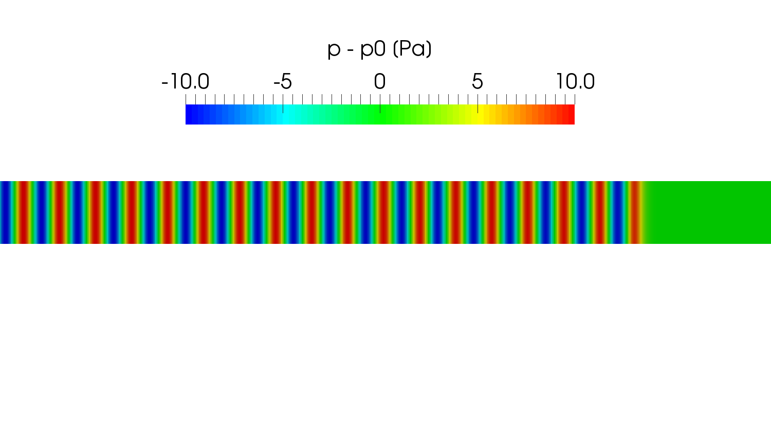
We consider an oscillatory motion with small amplitude in a compressible fluid as shown in the following picture. It shows the distribution of the sound pressure (acoustic pressure) that is defined as the local pressure deviation from the equilibrium pressure \(p_0\) caused by the sound wave propagating from left to right direction.
Since we now consider small oscillations, we can write the local pressure \(p\) and density \(\rho\) in the form
\begin{align}
p &= p_0 + p^{´}, \tag{1a} \label{eq:pressure} \\
\rho &= \rho_0 + \rho^{´}, \tag{1b} \label{eq:density}
\end{align}
where \(p_0\) and \(\rho_0\) are the constant equilibrium pressure and density and \(p^{´}\) and \(\rho^{´}\) are their variations in the sound wave (\(p^{´} \ll p_0, \rho^{´} \ll \rho_0\)), so the above figure is the contour of \(p^{´}\).
We hereafter ignore the fluid viscosity so that only the effect of compressibility is taken into account. Then, the governing equations of the fluid flow is the continuity equation
\begin{align}
\frac{\partial \rho}{\partial t} + \nabla \cdot (\rho \boldsymbol{u}) = 0 \tag{2} \label{eq:continuity}
\end{align}
and the Euler’s equation
\begin{align}
\frac{\partial \boldsymbol{u}}{\partial t} + (\boldsymbol{u} \cdot \nabla)\boldsymbol{u} + \frac{1}{\rho}\nabla p = 0 \tag{3} \label{eq:euler}
\end{align}
where \(\boldsymbol{u}\) is the velocity field. Substituting the eqns. \eqref{eq:pressure} and \eqref{eq:density} into the governing equations and neglecting small quantities of the second order, we get
\begin{align}
\frac{\partial \rho^{´}}{\partial t} + \rho_0 \nabla \cdot \boldsymbol{u} = 0, \tag{4} \label{eq:continuity2}
\end{align}
and
\begin{align}
\frac{\partial \boldsymbol{u}}{\partial t} + \frac{1}{\rho_0} \nabla p^{´} = 0. \tag{5} \label{eq:euler2}
\end{align}
We notice that a sound wave in an ideal fluid is adiabatic and the following relationship holds between the small changes in the pressure and density
\begin{align}
p^{´} = \left(\frac{\partial p}{\partial \rho} \right)_s \rho^{´} \tag{6} \label{eq:adiabatic}
\end{align}
where the subscript s denotes that the partial derivative is taken at constant entropy. Substituting it into \eqref{eq:continuity2}, we get
\begin{align}
\frac{\partial p^{´}}{\partial t} + \rho_0 \left(\frac{\partial p}{\partial \rho} \right)_s \nabla \cdot \boldsymbol{u} = 0. \tag{7} \label{eq:continuity3}
\end{align}
If we introduce the velocity potential \(\boldsymbol{u} = \nabla \phi\), we can derive the relationship between \(p^{´}\) and the potential \(\phi\) from \eqref{eq:euler2}
\begin{align}
p^{´} = -\rho_0 \frac{\partial \phi}{\partial t}. \tag{8} \label{eq:pandphi}
\end{align}
We then obtain the following wave equation from \eqref{eq:continuity3}
\begin{align}
\frac{\partial^2 \phi}{\partial t^2} – c^2 \Delta \phi = 0 \tag{9} \label{eq:waveEqn}
\end{align}
where \(c\) is the speed of sound in an ideal fluid
\begin{align}
c = \sqrt{\left(\frac{\partial p}{\partial \rho} \right)_s}. \tag{10} \label{eq:soundSpeed}
\end{align}
Applying the gradient operator to \eqref{eq:waveEqn}, we find that the each of the three components of the velocity \(\boldsymbol{u}\) satisfies an equation having the same form, and on differentiating \eqref{eq:waveEqn} with respect to time we see that the pressure \(p^{´}\) (and therefore \(\rho^{´}\)) also satisfies the wave equation.
– Landau and Lifshitz, Fluid Mechanics
In a travelling plane wave,
we find
\begin{align}
u_x = \frac{p^{´}}{\rho_0 c}. \tag{11} \label{eq:uxandp}
\end{align}Substituting here from \eqref{eq:adiabatic} \(p^{´} = c^2 \rho^{´}\), we find the relation between the velocity and the density variation:
\begin{align}
u_x = \frac{c \rho^{´}}{\rho_0}. \tag{12} \label{eq:uxandrho}
\end{align}– Landau and Lifshitz, Fluid Mechanics
This book is freely accessible from the link.
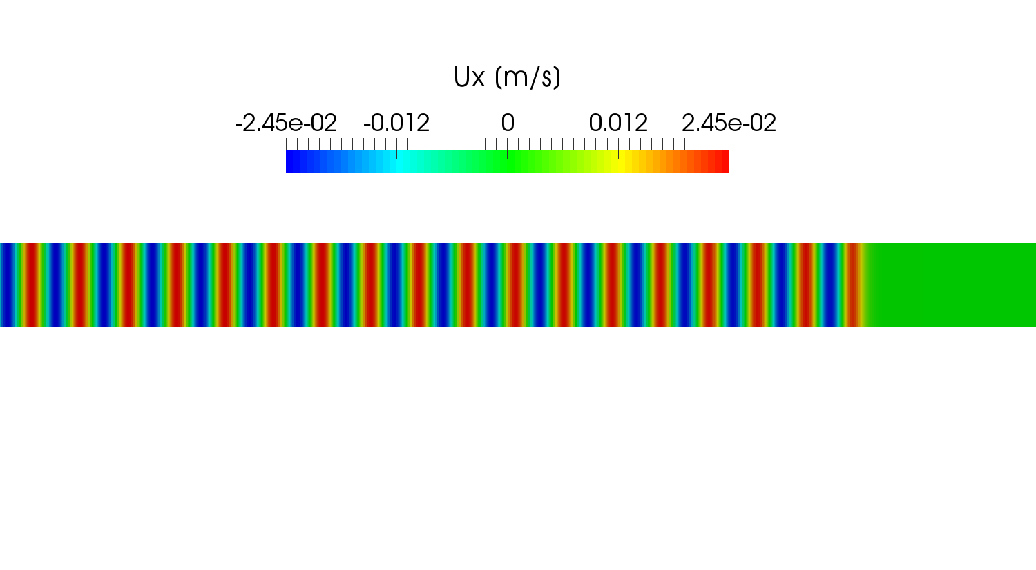
The following picture shows the velocity distribution \(u_x\) calculated using a compressible solver in OpenFOAM at the time corresponding to the pressure variation shown in the above picture. We can calculate the velocity using \eqref{eq:uxandp}
\begin{align}
u_x = \frac{10}{1.2 \times 340} = 0.0245 [m/s]
\end{align}
and it is in good agreement with the result obtained using OpenFOAM.
Computational Aeroacoustics (CAA) part1
This is the first in a series of posts about the computational aeroacoustics that is abbreviated as CAA. Aeroacoustics is mainly concerned with the generation of sound or noise through a fluid flow. Familiar examples are
- Aeolian tone
- Edge tone
- Cavity tone.
They can be studied by both experimental and computational methods. In an experimental approach, the aerodynamically generated sound is measured in the anechoic chamber that is designed to prevent reflections of sound on the wall, making the room echo-free. The following video created by Microsoft will help us to understand the structure of it.
The computational techniques for simulating flow-generated noise can be classified into two broad categories:
| Direct Approaches |
The governing equations of the compressible fluid flow is the compressible Navier-Stokes equations and they also describe the generation and propagation of acoustic noise, so we can solve the computational aeroacoustics problems by solving the transient compressible Navier-Stokes equations both in the source region where the flow disturbances generate noise and propagation region where the generated acoustic waves propagate. Acoustic waves have to be resolved in both regions so that the noise can be accurately simulated at observation locations. However, the solution of the Navier–Stokes equations with fine mesh over large domains to determine farfield noise is computationally very expensive.
As is the case in the experimental approaches, it is essential to prevent the reflection of the acoustic waves on the artificially truncated boundary (i.e. it does not stretch to infinity) of the computational domain in order to obtain an accurate result. A variety of numerical techniques have been developed for this purpose:
- Navier-Stokes Characteristic Boundary Conditions (NSCBC)
- Artificial dissipation and damping in an absorbing zone
- Grid stretching and numerical filtering in a “sponge layer” or “exit zone”
- Perfectly matched layer (PML)
In OpenFOAM, acousticDampingSource is categorized into Ⅱ and the waveTransmissive boundary condition is an approximation of NSCBC.
| Hybrid Approaches (Acoustic Analogy) |
David P. Lockard and Jay H. Casper [1] states that:
The physics-based, airframe noise prediction methodology under investigation is a hybrid of aeroacoustic theory and
computational fluid dynamics (CFD). The near-field aerodynamics associated with an airframe component are simulated to obtain the source input to an acoustic analogy that propagates sound to the far field. The acoustic analogy employed within this current framework is that of Ffowcs Williams and Hawkings, who extended the analogies of Lighthill and Curle to the formulation of aerodynamic sound generated by a surface in arbitrary motion.
- Lighthill’s analogy
Lighthill derived the following wave equation \eqref{eq:Lighthill} from the compressible Navier-Stokes equations:
\begin{align}
\frac{\partial^2 \rho}{\partial t^2} – c_0^2 \nabla^2 \rho = \frac{\partial^2 T_{ij}}{\partial x_i \partial x_j}, \tag{1} \label{eq:Lighthill}
\end{align}
where the so-called Lighthill (turbulence) stress tensor is expressed as
\begin{align}
T_{ij} = \rho u_i u_j + \left( p-c_0^2 \rho \right)\delta_{ij} -\mu \left(\frac{\partial u_i}{\partial x_j} + \frac{\partial u_j}{\partial x_i} – \frac{2}{3}\delta_{ij}\frac{u_k}{x_k} \right), \tag{2} \label{eq:Tij}
\end{align}
\(\delta_{ij}\) is the Kronecker delta and \(c_0\) is the speed of sound in the medium in its equilibrium state.
- Curle’s analogy
The existence of the objects (solid walls) is not considered in the Lighthill’s theory and Curle developed the theory so that it can be dealt with. The density variation at the observer location \(\boldsymbol{x}\) is calculated from the following equation \eqref{eq:Curle}
\begin{align}
\acute{\rho}(\boldsymbol{x}, t) &= \rho(\boldsymbol{x}, t)\;- \rho_0 \\
&=\frac{1}{4 \pi c_0^2} \frac{\partial^2}{\partial x_i \partial x_j} \int_{V}\frac{[T_{ij}]}{r}dV – \frac{1}{4 \pi c_0^2} \frac{\partial}{\partial x_i}\int_{S}\frac{[P_i]}{r}dS, \tag{3} \label{eq:Curle}
\end{align}
where
\begin{align}
P_i = -n_j \{ \delta_{ij}p -\mu \left(\frac{\partial u_i}{\partial x_j} + \frac{\partial u_j}{\partial x_i} – \frac{2}{3}\delta_{ij}\frac{u_k}{x_k} \right) \}, \tag{4} \label{eq:Pi}
\end{align}
\(r\) is the distance between the receiver \(\boldsymbol{x}\) and the source position \(\boldsymbol{y}\) in \(V\) (or on \(S\)) and the operator [] denotes evaluation at the retarded time \(t-r/c_0\).
- Ffowcs-Williams and Hawkings (FW-H) analogy
In the following video, we can watch the lecture by James Lighthill and John Ffowcs Williams !
| References (English) |
- [1] Permeable Surface Corrections for Ffowcs Williams and Hawkings Integrals
- [2] CFD Online – Acoustic Solver with openfoam
- [3] WIKIBOOKS – Engineering Acoustics/Analogies in aeroacoustics
| References (Japanese) |
- [4] 加藤千幸,大規模数値流体解析による流体音の予測
- [5] 飯田明由,送風機(ファン)の騒音発生メカニズムと低減・静粛化対策とその事例
- [6] 大嶋拓也,流れ中の柱状物体列から発生する空力音の数値予測に関する研究
- [7] Newsletters Nagare Dec. issue 2010
fvOptions meanVelocityForce
| An Example Usage of meanVelocityForce |
|
1 2 3 4 5 6 7 8 9 10 11 12 13 14 15 16 17 18 19 20 21 22 23 24 25 26 27 28 29 30 31 32 33 34 |
/*--------------------------------*- C++ -*----------------------------------*\ | ========= | | | \\ / F ield | OpenFOAM: The Open Source CFD Toolbox | | \\ / O peration | Version: dev | | \\ / A nd | Web: www.OpenFOAM.org | | \\/ M anipulation | | \*---------------------------------------------------------------------------*/ FoamFile { version 2.0; format ascii; class dictionary; location "constant"; object fvOptions; } // * * * * * * * * * * * * * * * * * * * * * * * * * * * * * * * * * * * * * // momentumSource { type meanVelocityForce; active yes; meanVelocityForceCoeffs { selectionMode all; fields (U); Ubar (0.1335 0 0); relaxation 1.0; } } // ************************************************************************* // |
- fields: [Required] Name of the velocity field
- Ubar: [Required] Desired mean velocity
- relaxation: [Optional] Relaxation factor (default = 1.0)
- selectionMode: [Required] Domain the source is applied (all/cellSet/cellZone/points)
The parameter name fields has been changed from fieldNames in the latest version as described in this page.
The meanVelocityForce fvOptions calculates a momentum source so that the volume averaged velocity \eqref{eq:magUbarAve} in the whole computational domain (all) or a part of domain specified using cellSet or cellZone reaches the desired mean velocity Ubar.
\begin{align}
\frac{\sum_{i}^{} \left(\frac{\bar{\boldsymbol{u}}}{|\bar{\boldsymbol{u}}|} \cdot \boldsymbol{u}_i \right)V_i}{\sum_{i}^{} V_i}, \tag{1} \label{eq:magUbarAve}
\end{align}
where the summation is over the cells that belong to the user-specified domain, \(\bar{\boldsymbol{u}}\) is Ubar, \(\boldsymbol{u}_i\) is the velocity in the i-th cell and \(V_i\) is the volume of the i-th cell.
| patchMeanVelocityForce |
The patchMeanVelocityForce fvOptions is also available to specify the desired mean velocity on a patch instead of the volumetric average \eqref{eq:magUbarAve}.
|
1 2 3 4 5 6 7 8 9 10 11 12 13 14 15 |
momentumSource { type patchMeanVelocityForce; active yes; patchMeanVelocityForceCoeffs { selectionMode all; fields (U); Ubar (0.1335 0 0); patch inout1_half0; relaxation 1.0; } } |
| Tutorial |
| Source Code |
In the case of pimpleFoam, we can find three lines related to the fvOptions as shown in the following code (UEqn.H):
|
1 2 3 4 5 6 7 8 9 10 11 12 13 14 15 16 17 18 19 20 21 22 23 24 |
// Solve the Momentum equation MRF.correctBoundaryVelocity(U); tmp<fvVectorMatrix> tUEqn ( fvm::ddt(U) + fvm::div(phi, U) + MRF.DDt(U) + turbulence->divDevReff(U) == fvOptions(U) ); fvVectorMatrix& UEqn = tUEqn.ref(); UEqn.relax(); fvOptions.constrain(UEqn); if (pimple.momentumPredictor()) { solve(UEqn == -fvc::grad(p)); fvOptions.correct(U); } |
In what follows, we will take a closer look at each of three highlighted lines when the meanVelocityForce fvOptions is used. The source files of this class are in src/fvOptions/sources/derived/meanVelocityForce.
- l. 11
The addSup function is called from l.11 in UEqn.H when discretizing the momentum equation and source term Su is added to the equation.
|
190 191 192 193 194 195 196 197 198 199 200 201 202 203 204 205 206 207 208 209 210 211 212 213 214 215 216 217 218 219 220 221 222 223 224 225 226 |
void Foam::fv::meanVelocityForce::addSup ( fvMatrix<vector>& eqn, const label fieldi ) { DimensionedField<vector, volMesh> Su ( IOobject ( name_ + fieldNames_[fieldi] + "Sup", mesh_.time().timeName(), mesh_, IOobject::NO_READ, IOobject::NO_WRITE ), mesh_, dimensionedVector("zero", eqn.dimensions()/dimVolume, Zero) ); scalar gradP = gradP0_ + dGradP_; UIndirectList<vector>(Su, cells_) = flowDir_*gradP; eqn += Su; } void Foam::fv::meanVelocityForce::addSup ( const volScalarField& rho, fvMatrix<vector>& eqn, const label fieldi ) { this->addSup(eqn, fieldi); } |
- l. 17
The constrain function is called from l.17 in UEqn.H. The if loop is true in the first iteration and else loop is executed for the other iterations to initialize and update the volScalarField defined as the reciprocal of the diagonal coefficients.
|
229 230 231 232 233 234 235 236 237 238 239 240 241 242 243 244 245 246 247 248 249 250 251 252 253 254 255 256 257 258 259 260 |
void Foam::fv::meanVelocityForce::constrain ( fvMatrix<vector>& eqn, const label ) { if (rAPtr_.empty()) { rAPtr_.reset ( new volScalarField ( IOobject ( name_ + ":rA", mesh_.time().timeName(), mesh_, IOobject::NO_READ, IOobject::NO_WRITE ), 1.0/eqn.A() ) ); } else { rAPtr_() = 1.0/eqn.A(); } gradP0_ += dGradP_; dGradP_ = 0.0; } |
- l. 23
As the average velocity magUbarAve \eqref{eq:magUbarAve} reaches a user-specified value Ubar, the pressure gradient increment dGradP_ needed to adjust the average velocity converges to 0.
|
148 149 150 151 152 153 154 155 156 157 158 159 160 161 162 163 164 165 166 167 168 169 170 171 172 173 174 175 176 177 178 179 180 181 182 183 184 185 186 187 |
void Foam::fv::meanVelocityForce::correct(volVectorField& U) { const scalarField& rAU = rAPtr_(); // Integrate flow variables over cell set scalar rAUave = 0.0; const scalarField& cv = mesh_.V(); forAll(cells_, i) { label celli = cells_[i]; scalar volCell = cv[celli]; rAUave += rAU[celli]*volCell; } // Collect across all processors reduce(rAUave, sumOp<scalar>()); // Volume averages rAUave /= V_; scalar magUbarAve = this->magUbarAve(U); // Calculate the pressure gradient increment needed to adjust the average // flow-rate to the desired value dGradP_ = relaxation_*(mag(Ubar_) - magUbarAve)/rAUave; // Apply correction to velocity field forAll(cells_, i) { label celli = cells_[i]; U[celli] += flowDir_*rAU[celli]*dGradP_; } scalar gradP = gradP0_ + dGradP_; Info<< "Pressure gradient source: uncorrected Ubar = " << magUbarAve << ", pressure gradient = " << gradP << endl; writeProps(gradP); } |
Introduction of Open CAE Community in Japan
I heard that Japan’s contribution to the open source CAE communities in the world is limited. I’m afraid that it is the case but many lively activities are actually performed in Japanese communities. In this blog post, I will try to introduce some interesting topics so that the users around the world know what has been going on in Japan.
In Japan, the Open CAE Society of Japan was set up on 9 November, 2009. This general incorporated association has held the Open CAE symposium annually and hands-on training courses several times each year about OpenFOAM, Salome-Meca, and ParaView among other things in many parts of the nation. The number of participants in the annual symposium exceeds 100 in each year.
- Open CAE Symposium 2010
- Open CAE Symposium 2011
- Open CAE Symposium 2012@Gifu
- Open CAE Symposium 2013@Osaka
- Open CAE Symposium 2014@Tokyo
- Open CAE Symposium 2015@Toyama
- Open CAE Symposium 2016@Tokyo to be held on Nov. 2016
You can get the latest news on this year’s symposium from the twitter account(@OpenCae2016).
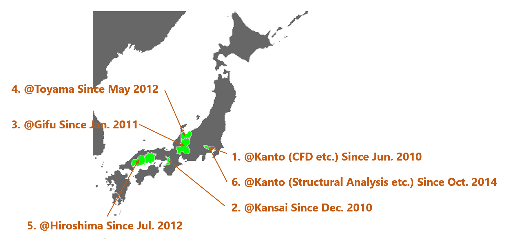
The association additionally gives support to the local study meetings (Open CAE “Benkyou Kai” in Japanese) where many willing industrial and student users get together about once a month to talk to each other about the progress of their simulations of interest and promote friendship between the users. These meetings are actively held in many places in Japan as illustrated in the following figure.
Their styles of meetings are different depending on the area, particularly between Kansai and Kanto as described in the post Japan’s bitterest feud: Kansai vs. Kanto (CNN DISCOVER JAPAN):
In Japan, a rivalry that can be just as fierce lies between the eastern Kanto region and western Kansai region, both on the main island of Honshu.
Kanto is home to the country’s modern capital of Tokyo and surrounding cities, including Yokohama, Chiba and Saitama.
Kansai is home to its historic capital of Osaka, as well as Kyoto, Kobe, Nara.
The cultural contention between the two is so longstanding, and entertaining, that it’s regularly discussed on Japanese TV shows.
You can watch the following movie to find out one of the most interesting and unique examples of their activities. In Kansai group, they build experimental equipments and carry out experiments to improve their understanding of the simulation results.
You can also find the presentation materials they have created in the following links. Almost all the participants are Japanese, so their materials are written in Japanese.
- OpenCAE user group@KANTO
- OpenCAE user group@KANSAI
- OpenCAE user group@GIFU
- OpenCAE user group@TOYAMA
The last topic in this post is about a new book. The first Japanese OpenFOAM book about the numerical analysis of heat transfer and fluid flow using OpenFOAM will be published in this month. It is written by the most famous Japanese blogger about OpenFOAM.
I will continue to report the latest news on the community in Japan.
Please wait till the next update! 🙂
P.S. Please tell me your opinions on how to make use of these Japanese materials in the world community!
Bandwidth, Profile and Frontwidth of Matrix
When we discretize the partial differential equations using the Finite Volume Method (FVM), we get sets of linear algebraic equations with large sparse coefficient matrices that are solved using iterative or direct methods. There is renumberMesh utility in OpenFOAM that is used to reduce the bandwidth of the coefficient matrices by renumbering the cell label list.
The bandwidth is not a special term in OpenFOAM but it is a general concept in the field of solving linear systems of equations. In this blog post, I will try to give a description of it and other important terms such as profile and frontwidth.
Keywords: bandwidth, profile, frontwidth, renumberMesh
| Definitions of bandwidth, profile and frontwidth |
The definitions of these terms are clearly described in [1]. Let \(A\) be an \(N\) by \(N\) matrix with symmetric zero-nonzero structure, i.e. , \(a_{ij} \neq 0\) if and only if \(a_{ji} \neq 0\).
The \(i\)-th bandwidth of \(A\) is:
\begin{align}
\beta_i(A) = i \; – \; {\rm min}\{ j \; | \; a_{ij} \neq 0\}. \tag{1} \label{eq:ithBandwidth}
\end{align}The bandwidth of \(A\) is defined by
\begin{align}
\beta = \beta(A) &= {\rm max} \{ \beta_i(A) \; | \; 1 \leq i \leq N\} \\
&= {\rm max} \{ |i-j| \; | \; a_{ij} \neq 0 \}. \tag{2} \label{eq:Bandwidth}
\end{align}The quantity \(|Env(A)|\) is called the profile or the envelope size of \(A\), and is defined by:
\begin{align}
|Env(A)| = \sum_{i=1}^{N} \beta_i(A). \tag{4} \label{eq:Profile}
\end{align}Another quantity called frontwidth is defined by the number of rows of the envelope of \(A\) which intersect column \(i\).
\begin{align}
\omega_i(A) = \{ k \; | \; k > i \; and \; \exists l \leq i \; s.t. \; a_{kl} \neq 0 \} \tag{5} \label{eq:frontwidth}
\end{align}To estimate factorization time, a quantity called root mean square frontwidth is introduced by [2]. This quantity is given by:
\begin{align}
f = \sqrt{\frac{1}{N} \left( \sum_{i=1}^{N} \omega_i^2 \right)}. \tag{8} \label{eq:rmsFrontwidth}
\end{align}
| Output of renumberMesh utility |
When the renumberMesh utility is executed, the following data is reported to the screen.
|
1 2 3 4 5 6 7 8 9 10 11 12 13 14 15 16 17 18 19 20 21 22 23 24 25 26 27 28 |
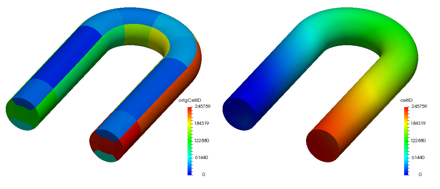
Create time Create mesh for time = 0 Mesh size: 245760 Before renumbering : band : 217487 profile : 2793999079 rms frontwidth : 12694.49013 Renumber according to renumberMeshDict Writing renumber maps (new to old) to polyMesh. Selecting renumberMethod CuthillMcKee After renumbering : band : 978 profile : 226514746 rms frontwidth : 932.0721888 Writing mesh to "1" Written current cellID and origCellID as volScalarField for use in postprocessing. End |
Here, the band, profile and rms frontwidth correspond to \eqref{eq:Bandwidth}, \eqref{eq:Profile} and \eqref{eq:rmsFrontwidth}, respectively. We can confirm that they all decreased after renumbering the cell label using the Cuthill-McKee (CM) algorithm. The distributions of cell labels are visually compared between before and after reordering operations in Figure 1.
| Source code of renumberMesh utility |
|
116 117 118 119 120 121 122 123 124 125 126 127 128 129 130 131 132 133 134 135 136 137 138 139 140 141 142 143 144 145 146 147 148 149 150 151 152 153 154 155 156 157 158 159 160 161 162 163 |
// Calculate band of matrix void getBand ( const bool calculateIntersect, const label nCells, const labelList& owner, const labelList& neighbour, label& bandwidth, scalar& profile, // scalar to avoid overflow scalar& sumSqrIntersect // scalar to avoid overflow ) { labelList cellBandwidth(nCells, 0); scalarField nIntersect(nCells, 0.0); forAll(neighbour, facei) { label own = owner[facei]; label nei = neighbour[facei]; // Note: mag not necessary for correct (upper-triangular) ordering. label diff = nei-own; cellBandwidth[nei] = max(cellBandwidth[nei], diff); } bandwidth = max(cellBandwidth); // Do not use field algebra because of conversion label to scalar profile = 0.0; forAll(cellBandwidth, celli) { profile += 1.0*cellBandwidth[celli]; } sumSqrIntersect = 0.0; if (calculateIntersect) { forAll(nIntersect, celli) { for (label colI = celli-cellBandwidth[celli]; colI <= celli; colI++) { nIntersect[colI] += 1.0; } } sumSqrIntersect = sum(Foam::sqr(nIntersect)); } } |
The getBand function is called from the main function. The variables band, profile and rmsFrontwidth represent \eqref{eq:Bandwidth}, \eqref{eq:Profile} and \eqref{eq:rmsFrontwidth}, respectively.
|
651 652 653 654 655 656 657 658 659 660 661 662 663 664 665 666 667 668 669 670 671 672 673 674 675 676 677 678 679 680 681 682 683 684 685 686 687 688 |
const bool readDict = args.optionFound("dict"); const bool doFrontWidth = args.optionFound("frontWidth"); const bool overwrite = args.optionFound("overwrite"); label band; scalar profile; scalar sumSqrIntersect; getBand ( doFrontWidth, mesh.nCells(), mesh.faceOwner(), mesh.faceNeighbour(), band, profile, sumSqrIntersect ); reduce(band, maxOp<label>()); reduce(profile, sumOp<scalar>()); scalar rmsFrontwidth = Foam::sqrt ( returnReduce ( sumSqrIntersect, sumOp<scalar>() )/mesh.globalData().nTotalCells() ); Info<< "Mesh size: " << mesh.globalData().nTotalCells() << nl << "Before renumbering :" << nl << " band : " << band << nl << " profile : " << profile << nl; if (doFrontWidth) { Info<< " rms frontwidth : " << rmsFrontwidth << nl; } |
| References |
- [1] A NEW FAST METHOD OF PROFILE AND WAVEFRONT REDUCTION FOR CYLINDRICAL STRUCTURES IN FINITE ELEMENTS METHOD ANALYSIS (accessed 2016-05-29)
- [2] A FORTRAN PROGRAM FOR PROFILE AND WAVEFRONT REDUCTION (accessed 2016-05-29)
Introduction to laplacianFoam and simple validation calculation
In this blog post, I will try to give a description of the governing equation of the laplacianFoam in OpenFOAM that solves a simple Laplace equation, e.g. for thermal diffusion in a solid.
| Governing Equation |
The heat conduction equation is given by the following equation:
\begin{align}
\frac{\partial T}{\partial t} = \frac{1}{\rho c_p} \nabla \cdot \left(k \nabla T\right) + \frac{q}{\rho c_p}, \tag{1} \label{eq:conductionEqn}
\end{align}
where \(T\;{\rm [ K]}\) is the absolute temperature field, \(\rho\;{\rm [kg/m^3]}\) is the density field, \(q\;{\rm [W/m^3]}\) is the rate of energy generation per unit volume, \(k\;{\rm [W/(m\cdot K)]}\) is the thermal conductivity and \(c_p\;{\rm [J/(kg\cdot K)]}\) is the specific heat at constant pressure.
If the heat capacity \(\rho c_p\) is spatially uniform, the Eq. \eqref{eq:conductionEqn} can be transformed into the following form irrespective of whether the thermal conductivity \(k\) is spatially uniform or not:
\begin{align}
\frac{\partial T}{\partial t} = \nabla \cdot \left(\alpha \nabla T\right) + \frac{q}{\rho c_p}, \tag{2} \label{eq:conductionEqn2}
\end{align}
where \(\alpha = k/\rho c_p\;{\rm [m^2/s]}\) is the thermal diffusivity.
The laplacianFoam (in OpenFOAM-4.x and earlier versions) doesn’t consider the heat generation and the implemented equation is
\begin{align}
\frac{\partial T}{\partial t} = \nabla \cdot \left(\alpha \nabla T\right), \tag{3} \label{eq:laplacianFoam}
\end{align}
but the solver in the latest development version supports the fvOptions so that we can solve \eqref{eq:conductionEqn2} and specify a volumetric heat source.
We can find the Eq. \eqref{eq:conductionEqn2} solved in laplacianFoam.C.
|
58 59 60 61 62 63 64 65 66 67 68 69 70 |
while (simple.correctNonOrthogonal()) { fvScalarMatrix TEqn ( fvm::ddt(T) - fvm::laplacian(DT, T) == fvOptions(T) ); fvOptions.constrain(TEqn); TEqn.solve(); fvOptions.correct(T); } |
The variable DT represents the thermal diffusivity \(\alpha\) and it is specified in the constant/transportProperties file.
|
1 2 3 4 5 6 7 8 9 10 11 12 13 14 |
FoamFile { version 2.0; format ascii; class dictionary; location "constant"; object transportProperties; } // * * * * * * * * * * * * * * * * * * * * * * * * * * * * * * * * * * * * * // DT DT [0 2 -1 0 0 0 0] 4e-05; // thermal diffusivity m^2/s // ************************************************************************* // |
| Comparison with Analytical Solution |
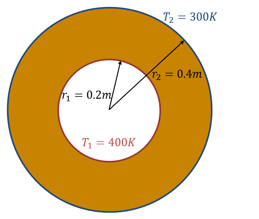
We consider the steady state problem of source-free heat conduction in a concentric cylinder whose inner and outer walls are maintained at constant temperature of 400 K and 300 K respectively. This problem can be analytically solved and the following relation holds for the temperature distribution in the radial direction \(T(r)\):
\begin{align}
\frac{T_1 – T(r)}{T_1 – T_2} = \frac{\ln{(r/r_1)}}{\ln{(r_2/r_1)}}, \tag{4} \label{eq:cylinderT}
\end{align}
where the subscripts 1 and 2 indicate the values at the inner and outer walls respectively shown in Figure 1.
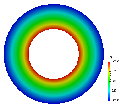
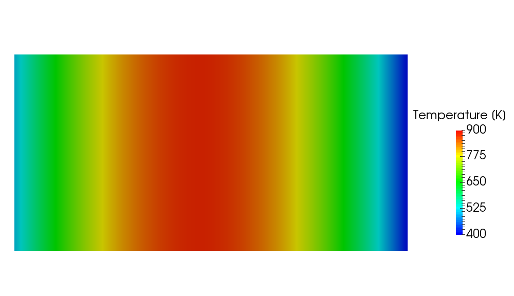
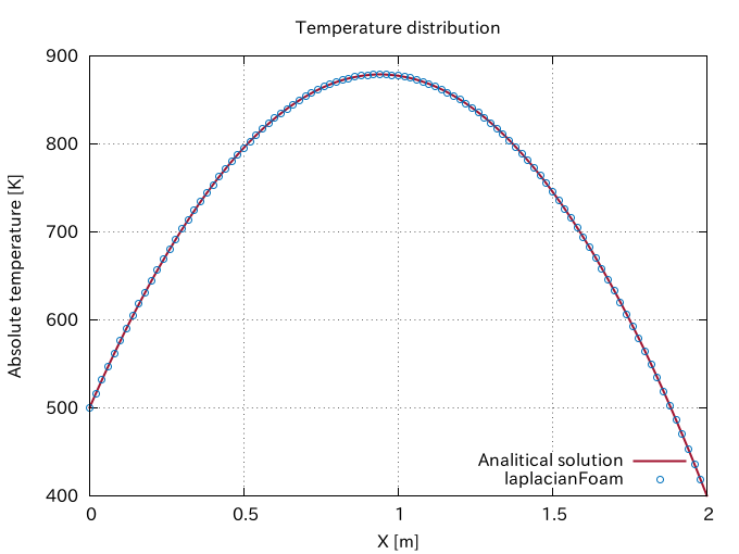
The temperature distribution obtained using laplacianFoam is shown in Figure 2 and the comparison between the numerical and analytical solutions is shown in Figure 3. The agreement with the analytical solution is good.

| Introduction of Source Term |
In the next post, I’ll deal with a simple example case to introduce how to specify a heat generation source term in laplacianFoam using the fvOptions functionality (scalarSemiImplicitSource).
Function Objects – histogram
OpenFOAM Version:
OpenFOAM-4.x
| Settings of histogram |
|
1 2 3 4 5 6 7 8 9 10 11 12 13 14 15 |
functions { temperatureHistogram { type histogram; functionObjectLibs ("libfieldFunctionObjects.so"); outputControl outputTime; // outputInterval 10; field T; nBins 10; min 300; max 310; setFormat gnuplot; } } |
| Histogram |
You can create a picture as shown below using Gnuplot with the input file generated by OpenFOAM. I replaced “with lines” with “with boxes” in the input command file to create this picture.

In the above picture, the first bin represents the following volume fraction:
\begin{align}
\frac{\sum_{celli}^{} \left( V_{celli}:\;300 \leq T_{celli} < 301\right)}{\sum_{celli}^{} \left( V_{celli}:\;min \leq T_{celli} < max\right)},
\end{align}
where \(V\) is the cell volume.
buoyantPimpleFoam and buoyantSimpleFoam in OpenFOAM
In this blog post, I will try to give a description of the governing equations of the following solvers in OpenFOAM for buoyant, turbulent flow of compressible fluids:
- buoyantPimpleFoam (Transient solver)
- buoyantSimpleFoam (Steady-state solver)
The solvers in OpenFOAM are named properly and comprehensibly so that the users can guess the meanings from their names 🙂
| Mass Conservation |
The mass conservation (continuity) equation of buoyantPimpleFoam is given by the following equation:
\begin{align}
\frac{\partial \rho}{\partial t} + \nabla \cdot \left( \rho \boldsymbol{u} \right) = 0, \tag{1} \label{eq:mass}
\end{align}
where \(\boldsymbol{u}\) is the velocity field and \(\rho\) is the density field. For the steady-state solver, the time derivative term is omitted.
| Momentum Conservation |
The momentum conservation equation of buoyantPimpleFoam is given by the following equation:
\begin{align}
\frac{\partial \left(\rho \boldsymbol{u} \right)}{\partial t} + \nabla \cdot \left(\rho\boldsymbol{u}\boldsymbol{u}\right) = &-\nabla p + \rho \boldsymbol{g} + \nabla \cdot \left(2 \mu_{eff} D \left( \boldsymbol{u} \right) \right) \\
&-\nabla \left( \frac{2}{3}\mu_{eff}\left(\nabla \cdot \boldsymbol{u} \right) \right), \tag{2} \label{eq:momentum}
\end{align}
where \(p\) is the static pressure field and \(\boldsymbol{g}\) is the gravitational acceleration. The effective viscosity \(\mu_{eff}\) is the sum of the molecular and turbulent viscosity and the rate of strain (deformation) tensor \(D\left(\boldsymbol{u}\right)\) is defined as \(D\left(\boldsymbol{u}\right) = \frac{1}{2}\left( \nabla \boldsymbol{u} + \left(\nabla \boldsymbol{u}\right)^{T} \right)\). As is the case in the continuity equation, the time derivative term is omitted in buoyantSimpleFoam.
In terms of the implementation in OpenFOAM, the pressure gradient and gravity force terms are rearranged in the following form:
\begin{align}
-\nabla p + \rho \boldsymbol{g}
&= -\nabla \left( p_{rgh} + \rho \boldsymbol{g} \cdot \boldsymbol{r} \right) + \rho \boldsymbol{g} \tag{3a}\\
&= -\nabla p_{rgh} – \left( \boldsymbol{g} \cdot \boldsymbol{r} \right) \nabla \rho \:- \rho \boldsymbol{g} + \rho \boldsymbol{g} \tag{3b} \\
&= -\nabla p_{rgh} – \left( \boldsymbol{g} \cdot \boldsymbol{r} \right) \nabla \rho, \tag{3c} \label{eq:prgh}
\end{align}
where \(p_{rgh} = p \;- \rho \boldsymbol{g} \cdot \boldsymbol{r}\) and \(\boldsymbol{r}\) is the position vector.
|
1 2 3 4 5 6 7 8 9 10 11 12 13 14 15 16 17 18 19 20 21 22 23 24 25 26 27 28 29 30 31 32 33 34 35 |
// Solve the Momentum equation MRF.correctBoundaryVelocity(U); fvVectorMatrix UEqn ( fvm::ddt(rho, U) + fvm::div(phi, U) + MRF.DDt(rho, U) + turbulence->divDevRhoReff(U) == fvOptions(rho, U) ); UEqn.relax(); fvOptions.constrain(UEqn); if (pimple.momentumPredictor()) { solve ( UEqn == fvc::reconstruct ( ( - ghf*fvc::snGrad(rho) - fvc::snGrad(p_rgh) )*mesh.magSf() ) ); fvOptions.correct(U); K = 0.5*magSqr(U); } |
In the above code, MRF stands for Multiple Reference Frame, which is one method for solving the problems including the rotating parts with the static mesh. This option is activated if constant/MRFProperties file exists. The line 11(fvOptions(rho, U)) is to add the user-specific source terms using fvOptions functionality.
| Energy Conservation |
We can choose either internal energy \(e\) or enthalpy \(h\) as the energy solution variable [3]. This selection is made according to energy keyword in thermophysicalProperties file.
|
1 2 3 4 5 6 |
thermoType { type heRhoThermo; ... energy sensibleEnthalpy or sensibleInternalEnergy; } |
For each variable, the energy conservation equations of buoyantPimpleFoam are given by the following equations:
- Enthalpy (sensibleEnthalpy)
\begin{align}
&\frac{\partial \left(\rho h \right)}{\partial t} + \nabla \cdot \left( \rho \boldsymbol{u} h \right) + \frac{\partial \left(\rho K \right)}{\partial t} + \nabla \cdot \left( \rho \boldsymbol{u} K \right) -\frac{\partial p}{\partial t} \\
&= \nabla \cdot \left( \alpha_{eff} \nabla h \right) + \rho \boldsymbol{u} \cdot \boldsymbol{g} \tag{4} \label{eq:energyH}
\end{align}
- Internal energy (sensibleInternalEnergy)
\begin{align}
&\frac{\partial \left(\rho e \right)}{\partial t} + \nabla \cdot \left( \rho \boldsymbol{u} e \right) + \frac{\partial \left(\rho K \right)}{\partial t} + \nabla \cdot \left( \rho \boldsymbol{u} K \right) + \nabla \cdot \left( p \boldsymbol{u} \right) \\
&= \nabla \cdot \left( \alpha_{eff} \nabla e \right) + \rho \boldsymbol{u} \cdot \boldsymbol{g} \tag{5} \label{eq:energyE}
\end{align}
where \(K \equiv |\boldsymbol{u}|^2/2\) is kinetic energy per unit mass and the enthalpy per unit mass \(h\) is the sum of the internal energy per unit mass \(e\) and the kinematic pressure \(h \equiv e + p/\rho\). We can get the following relations from this definition:
\begin{align}
\frac{\partial \left(\rho e \right)}{\partial t} = \frac{\partial \left(\rho h \right)}{\partial t} \;-\; \frac{\partial p}{\partial t}, \tag{6a} \\
\nabla \cdot \left( \rho \boldsymbol{u} e \right) = \nabla \cdot \left( \rho \boldsymbol{u} h \right) \;-\; \nabla \cdot \left( p \boldsymbol{u} \right). \tag{6b}
\end{align}
The effective thermal diffusivity \(\alpha_{eff}/\rho\) is the sum of laminar and turbulent thermal diffusivities:
\begin{align}
\alpha_{eff} = \frac{\rho \nu_t}{Pr_t} + \frac{\mu}{Pr} = \frac{\rho \nu_t}{Pr_t} + \frac{k}{c_p}, \tag{7} \label{eq:alphaEff}
\end{align}
where \(k\) is the thermal conductivity, \(c_p\) is the specific heat at constant pressure, \(\mu\) is the dynamic viscosity, \(\nu_t\) is the turbulent (kinematic) viscosity, \(Pr\) is the Prandtl number and \(Pr_t\) is the turbulent Prandtl number. The expression of the laminar thermal diffusivity changes depending on the selected thermodynamics package. As is the case in the momentum equation, the time derivative terms are omitted in buoyantSimpleFoam.
|
1 2 3 4 5 6 7 8 9 10 11 12 13 14 15 16 17 18 19 20 21 22 23 24 25 26 27 28 29 30 31 32 33 34 35 |
{ volScalarField& he = thermo.he(); fvScalarMatrix EEqn ( fvm::ddt(rho, he) + fvm::div(phi, he) + fvc::ddt(rho, K) + fvc::div(phi, K) + ( he.name() == "e" ? fvc::div ( fvc::absolute(phi/fvc::interpolate(rho), U), p, "div(phiv,p)" ) : -dpdt ) - fvm::laplacian(turbulence->alphaEff(), he) == rho*(U&g) + radiation->Sh(thermo) + fvOptions(rho, he) ); EEqn.relax(); fvOptions.constrain(EEqn); EEqn.solve(); fvOptions.correct(he); thermo.correct(); radiation->correct(); } |
The line 21 represents the contributions from the radiative heat transfer. The effective thermal diffusivity \(\alpha_{eff}\) \eqref{eq:alphaEff} is calculated in heThermo.C:
|
784 785 786 787 788 789 790 791 792 793 794 |
template<class BasicThermo, class MixtureType> Foam::tmp<Foam::volScalarField> Foam::heThermo<BasicThermo, MixtureType>::alphaEff ( const volScalarField& alphat ) const { tmp<Foam::volScalarField> alphaEff(this->CpByCpv()*(this->alpha_ + alphat)); alphaEff.ref().rename("alphaEff"); return alphaEff; } |
When solving for enthalpy \(h\), the pressure-work term \(dp/dt\) can be excluded by setting the dpdt option to no in thermophysicalProperties file [3]. The volScalarField \(dp/dt\) is defined and uniformly initialized to zero in createFields.H and updated in pEqn.H if this option is activated.
|
78 79 80 81 82 83 84 85 86 87 88 89 |
Info<< "Creating field dpdt\n" << endl; volScalarField dpdt ( IOobject ( "dpdt", runTime.timeName(), mesh ), mesh, dimensionedScalar("dpdt", p.dimensions()/dimTime, 0) ); |
|
69 70 71 72 |
if (thermo.dpdt()) { dpdt = fvc::ddt(p); } |
When the mesh is static, the fvc::absolute function does nothing as shown below:
|
187 188 189 190 191 192 193 194 195 196 197 198 199 200 201 |
Foam::tmp<Foam::surfaceScalarField> Foam::fvc::absolute ( const tmp<surfaceScalarField>& tphi, const volVectorField& U ) { if (tphi().mesh().moving()) { return tphi + fvc::meshPhi(U); } else { return tmp<surfaceScalarField>(tphi, true); } } |
| References |
[1] Energy Equation in OpenFOAM | CFD Direct
[2] OpenFOAM User Guide: 7.1 Thermophysical models | CFD Direct
[3] OpenFOAM 2.2.0: Thermophysical Modelling
Postprocessing with foamCalc utility
After the simulation has finished, you can do simple calculation, such as addition and subtraction, with the field data using foamCalc utility. The source code is located in the following directories:
- applications/utilities/postProcessing/foamCalc
- src/postProcessing/foamCalcFunctions.
| components |
$ foamCalc components U -latestTime
This example is to generate three component files Ux, Uy and Uz (volScalarField) from volVectorField U only at the latest time directory.
| mag |
$ foamCalc mag U
This example is to generate velocity magnitude field \(|\boldsymbol{U}|\) file magU at every existing time directory.
| magSqr |
$ foamCalc magSqr U
This example is to generate magnitude squared field \(|\boldsymbol{U}|^2\) file magSqrU at every existing time directory.
| addSubtract |
$ foamCalc addSubtract T subtract -value 273.15 -resultName Tdeg -time 5000
This example is to convert the temperature unit from Kelvin to degrees at time 5000. The generated file name can be specified using –resultName option.
| div |
$ foamCalc div phi
This example is to calculate the divergence of the flux field phi for the estimation of the continuity error of each cell for incompressible flow.
| interpolate |
$ foamCalc interpolate T -latestTime
This example it to generate surfaceScalarField interpolateT from volScalarField T using the interpolation scheme specified in the system/fvSchemes file.