Last Updated: May 5, 2019
When we solve a partial differential equation with a source term, we must pay attention to how to treat it numerically for better convergence. The SemiImplicitSource fvOption is available in OpenFOAM so that we can handle a linearized source term in numerically stable way.
Keywords
- Source term linearization
- SemiImplicitSource in OpenFOAM
| Source Term Linearization |
If the source term under consideration is a non-linear function of a conserved variable, the linearization of it is a fundamental approach to discretizing it in the finite volume method. This topic is precisely covered in the famous book “Numerical Heat Transfer and Fluid Flow” by Suhas V. Patankar:
In Section 4.2.5, the concept of the linearization of the source term was introduced. One of the basic rules (Rule 3) required that when the source term is linearized as
\begin{equation}
S = S_C + S_P \phi_P, \tag{7.6} \label{eq:sourceTerm}
\end{equation}the quantity \(S_P\) must not be positive. Now, we return to the topic of source-term linearization to emphasize that often source terms are the cause of divergence of iterations and that proper linearization of the source term frequently holds the key to the attainment of a converged solution.
Rule 3: Negative-slope linearization of the source term If we consider the coefficient definitions in Eqs. (3.18), it appears that, even if the neighbor coefficients are positive, the center-point coefficient \(a_P\) can become negative via the \(S_P\) term. Of course, the danger can be completely avoided by requiring that \(S_P\) will not be positive. Thus, we formulate Rule 3 as follows:
When the source term is linearized as \(\bar{S} = S_C + S_P T_P\), the coefficient \(S_P\) must always be less than or equal to zero.
| Linearized Source Specification for a Scalar Field in OpenFOAM |
In OpenFOAM, the linearized source terms can be specified using SemiImplicitSource fvOption. Its settings are described in the constant/fvOptions file.
|
1 2 3 4 5 6 7 8 9 10 11 12 13 14 15 16 17 18 19 20 21 22 23 24 25 26 27 28 29 30 31 32 33 34 35 36 |
/*--------------------------------*- C++ -*----------------------------------*\ | ========= | | | \\ / F ield | OpenFOAM: The Open Source CFD Toolbox | | \\ / O peration | Version: dev | | \\ / A nd | Web: www.OpenFOAM.org | | \\/ M anipulation | | \*---------------------------------------------------------------------------*/ FoamFile { version 2.0; format ascii; class dictionary; location "constant"; object fvOptions; } // * * * * * * * * * * * * * * * * * * * * * * * * * * * * * * * * * * * * * // heatSource { type scalarSemiImplicitSource; active true; scalarSemiImplicitSourceCoeffs { selectionMode all; // all, cellSet, cellZone, points cellSet c1; volumeMode specific; // absolute; injectionRateSuSp { T (0.1 0); } } } // ************************************************************************* // |
- selectionMode: [Required] Domain where the source is applied (all/cellSet/cellZone/points)
- injectionRateSuSp: [Required] Conserved variable name and two coefficients of linearized source term
|
1 2 3 4 |
injectionRateSuSp { variable_name (Sc Sp); } |
- volumemode: [Required] Choice of how to specify the two coefficients
– absolute: values are given as [variable]
– specific: values are given as [variable]/\({\rm m^3}\)
| Example 1. Heat Conduction with Heat Source |
Let’s consider a simple 1D heat conduction problem in a solid rod with a thermal energy generation per unit volume and time \(\dot{q}_v {\rm [W/m^3]}\). In this case, the steady heat conduction equation in 1D is given by
\begin{align}
\alpha \frac{d^2 T}{d x^2} + \frac{\dot{q}_v}{\rho c} = 0. \tag{1} \label{eq:conductionEqn}
\end{align}
Here, we assume that the thermal diffusivity \(\alpha {\rm [m^2/s]}\) is constant.
We can obtain the general solution for this equation \eqref{eq:conductionEqn} by integrating it twice.
\begin{equation}
T(x) = -\frac{S_C}{2\alpha}x^2 + C_1 x + C_2, \tag{2} \label{eq:generalSolution}
\end{equation}
where \(C_1\) and \(C_2\) are integration constants and we put \(S_C {\rm [K/s]} := \dot{q}_v/\rho c\). If we assume that the temperatures at both ends of the rod are maintained at constant temperatures \(T(0) = T_1, T(L) = T_2\), we can determine the values of two integration constants as
\begin{align}
C_2 &= T_1, \tag{3} \\
C_1 &= \frac{T_2 – T_1}{L} + \frac{S_C L}{2\alpha}. \tag{4}
\end{align}
Then, the temperature distribution in the rod is expressed by the following equation:
\begin{equation}
T(x) = -\frac{S_C}{2\alpha}x^2 + \left( \frac{T_2 – T_1}{L} + \frac{S_C L}{2\alpha} \right)x + T_1. \tag{5} \label{eq:solution}
\end{equation}
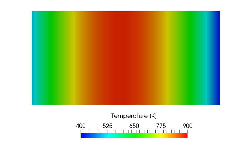
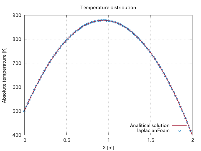
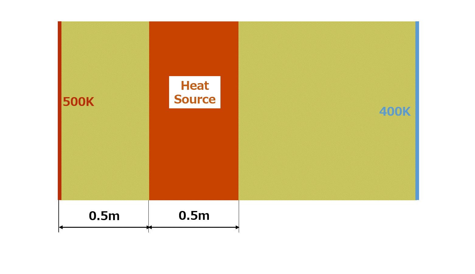
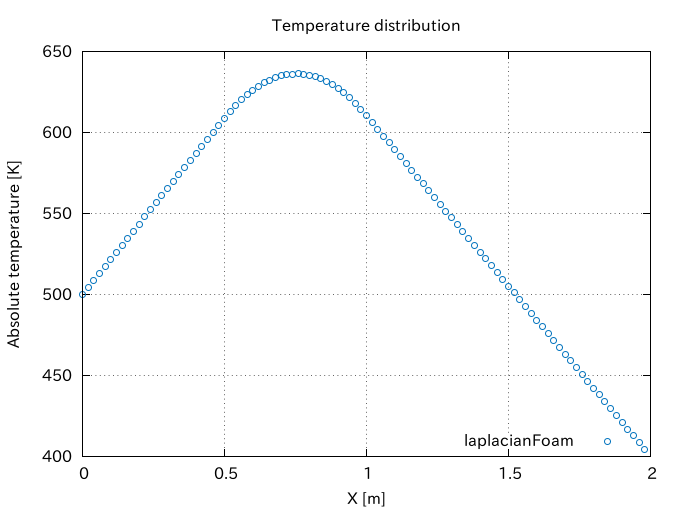
If we confine the heat source region to one-quarter of the whole region as shown in the following picture, the quadratic temperature distribution is limited to the region and the linear profile is obtained in the source free region.

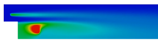
| Example 2. Passive Scalar Transport |
Thank you Fumiya for nice explanation! I was struggling to find out the reason for error in my case. I noticed in your post that “selectionMode and cellSet ” should be inside scalarSemiImplicitSourceCoeffs { … } and not outside that is inside heatSource { … } as mentioned in sample fvOption file at github.
Regards,
Amod
Thank you for this explanation! I was wondering if I could see your case (or just your fvOptions file) for example 2: Passive Scalar transport. I am working on a 2D problem and require a heat source for about 2 seconds (to simulate a lighter) to start combustion of a premixed jet.
I think I am having trouble calculating the right amount of heat to add and which selection mode to implement.
it is very useful i need more details about source term compilation in openfoam
thank a lot
Hello Fumiya, Thanks for all the help.
I am currenlty modelling free convection in a room with inlets, outlets and heat sources. I am using buoyantPimpleFoam to begin and further using buoyantSimpleFoam.
I’m setting a large volume with heat loads and have been forced to define h (sensible enthalpy?) instead of T. would you have any advice on how to set h considering my heat source is 10 w/m2?
Kind regards,
olivier
Thank you dear Fumiya
I tried to reporoduce the results above where the source term is specified everywhere in the computational domain but unfortuantely the analytical and the numerical results are very different.
In constant/transportProperties I used the following:
Dt = 1.0
In fvOptions, I used:
scalarSemiImplicitSourceCoeffs
{
selectionMode all;
volumeMode absolute;
injectionRateSuSp
{
T (100 0);
}
}
In the analytical formula, I used Sc = 100 and alpha = 100
What is wrong?
Thank you
Sorry, I fixed the problem by changing the volumeMode to specific.
what about if the source term is non-linear (dependent on temperature)?
Hi dear
Thanks for the useful information.
Do you have any idea how to consider a heat source in a region (in multi region case) while the temperature is kept at a constant value?
Regards
Mohammad
Hello thanks for the explanation
I am simulating a conjugate heat transfer problem, a simple case of a solid being cooled by a fluid. However no matter how much i increase the value of heat flux for the solid in fvOptions, the outlet air temperature or the temperature of the solid just does not change. it seems to be openfoam is just ignoring fvOptions file. Maximum value of temperature at the solid and outlet air temperature remains the same as the initial value and just does not change no matter how much i change heat flux value in fvOptions. Thanks for any advice. Regards
Dear Mr. Bineet and Fumiya
I have experienced exactly the same issue. I wonder if you have any improvement on this issue. It would be great if you can reply on this issue.
At last, I do appreciate this website information which is really helpful for the OF learners like me.
First, thank you for the excellent tutorial. It’s really simple and helpful
But I’m also facing the same issue- no matter how I increase the heat generation, the temperature is now affected at all. Is it wrong to assume that Sc=heat generation in Watt if the selection mode is absolute?
Hello dear thanks for such a nice explanation,
I’m going to add a source term (-Cb*(T-To)*g where Cb is thermal expension,g gravity,T temp,To initial temp) to viscoelasticFluidFoam solver i.e
tmp UEqn
(
fvm::ddt(U)
+ fvm::div(phi, U)
– visco.divTau(U)
);
kindly if any one could help me.
regards
idrees khan
Hi,
I’m solving chtMultiRegion case between fluid and solid region. Solid region is a sphere which is in the middle of the flow field. I wonder how can I add heat flux to the sphere? I’m open any advice.
Kind regards.
Said.