Reynolds-Averaged Navier-Stokes (RANS)

Last Updated: May 11, 2019

Keywords
Boussinesq approximation, closure problem, Reynolds averaging

Reynolds Average

It is computationally expensive to resolve the wide range of time and length scales observed in turbulent flows. We now consider decomposing a flow property \(f\), such as velocity and pressure, into a mean component \(\overline{f}\) and a fluctuating component \(f’\).
\begin{equation}
f(\boldsymbol{x}, t) = \overline{f}(\boldsymbol{x}, t) + f'(\boldsymbol{x}, t), \tag{1} \label{eq:decomposition}
\end{equation}
where \(\boldsymbol{x}\) is the position vector and \(t\) is time.

The Reynolds-averaged Navier-Stokes (RANS) turbulence models aim to solve the mean flow \(\overline{f}\) that changes more slowly in time and space than the original variable \(f\). The governing equations of the mean component will be derived later.

There are many averaging operations defined in mathematics but the RANS models use the Reynolds average. It is briefly described in the newly published textbook by Kajishima and Taira [1].

For the discussion in this chapter, let us redefine the averaging operation such that it satisfies
\begin{equation}
\overline{f’} = 0,\;\;\overline{f’ \overline{f}} = 0,\;\;\overline{\overline{f}} = \overline{f}. \tag{7.2} \label{eq:reave}
\end{equation}
These relations in Eq. \eqref{eq:reave} are referred to as the Reynolds-averaging laws. The ensemble average that satisfies these laws is called the Reynolds average. This conceptual averaging operation conveniently removes fluctuating components from the flow field variables without explicitly defining the spatial length scale used in the averaging operation.

The ensemble average that appears in the above definition is defined as (and usually denoted as \(\langle f \rangle\))
\begin{equation}
\langle f \rangle(\boldsymbol{x}, t) \equiv \lim_{N \to \infty}\frac{1}{N}\sum_{i=1}^{N}f_{i}(\boldsymbol{x}, t), \tag{2} \label{eq:ensembleAve}
\end{equation}
where \(f_i\) are the samples of \(f\) and \(N\) is the number of samples. In other words, it is the average of the instantaneous values of the property at a given point in space \(\boldsymbol{x}\) and time \(t\) over a large number of repeated identical experiments. In general, this ensemble average varies with space and time (time-dependent).

For the stationary random processes, we can define the time average \(f_T\):
\begin{equation}
f_{T}(\boldsymbol{x}) \equiv \frac{1}{T} \int_{0}^{T} f(\boldsymbol{x}, t) dt, \tag{3} \label{eq:timeAve}
\end{equation}
where \(T\) is the integration time. In the case of stationary random processes, the time averages equal the ensemble averages as stated in [3]:

if the signal is stationary, the time average defined by equation \eqref{eq:timeAve} is an unbiased estimator of the true average \(\langle f \rangle\). Moreover, the estimator converges to \(\langle f \rangle\) as the time becomes infinite; i.e., for stationary random processes
\begin{equation}
\langle f \rangle(\boldsymbol{x}) = \lim_{T \to \infty} \frac{1}{T} \int_{0}^{T} f(\boldsymbol{x}, t) dt, \tag{8.28} \label{eq:aveRelation}
\end{equation}
Thus the time and ensemble averages are equivalent in the limit as \(T \to \infty\), but only for a stationary random process.

Interested readers might want to search by the keyword ”ergodic hypothesis” on the relation between the ensemble and time averages.

RANS Equations

To Be Updated

Closure Problem – Reynolds Stress

The linear eddy viscosity models (LEVM) assume the linear stress-strain relationship and employ the eddy-viscosity concept (Boussinesq approximation) introduced by Joseph Valentin Boussinesq
\begin{equation}
-\rho\overline{u_i u_j} = \mu_t \left(\frac{\partial \overline{U}_i}{\partial x_j} + \frac{\partial \overline{U}_j}{\partial x_i} \right) -\frac{2}{3}\delta_{ij}\rho k. \tag{4} \label{eq:BoussinesqApprox}
\end{equation}

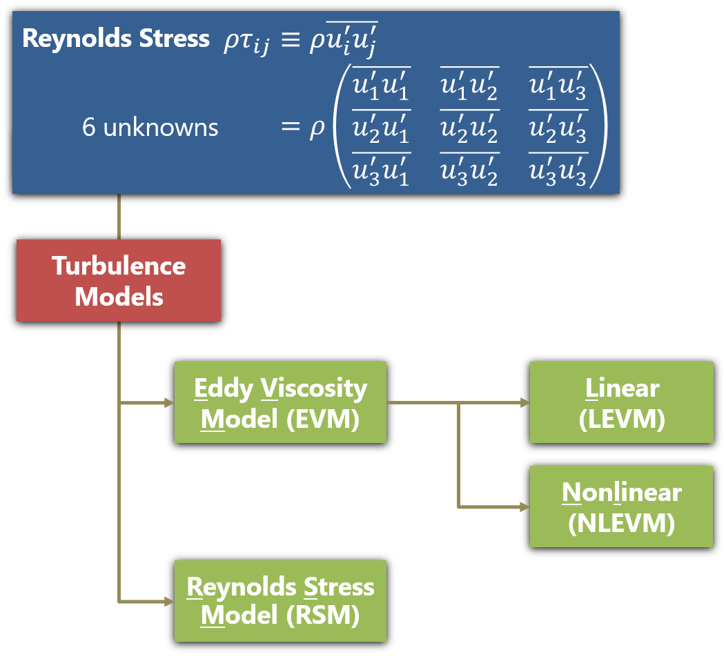
RANS Models in OpenFOAM

Linear Eddy Viscosity Model (LEVM)

• SpalartAllmaras
• kEpsilon
• realizableKE
• RNGkEpsilon
• LaunderSharmaKE
• kOmega
• kOmegaSST
• kkLOmega
• v2f

Nonlinear Eddy Viscosity Model (NLEVM)

• ShihQuadraticKE
• LienCubicKE

Reynolds Stress Model (RSM)

• LRR (Launder, Reece and Rodi)
• SSG (Speziale, Sarkar and Gatski)

Limitations of LEVM

Transition Models

• \(k\)-\(kl\)-\(\omega\)
• \(\gamma\)-\(Re_{\theta}\)

Differential Reynolds Stress model

• SSG/LRR-\(\omega\)
• JH-\(\omega^h\)

References

[1] T. Kajishima and K. Taira, Computational Fluid Dynamics: Incompressible Turbulent Flows. Springer, 2016.
[2] H. K. Versteeg and W. Malalasekera, An introduction to Computational Fluid Dynamics: The Finite Volume Method. Person Prentice Hall, 1995.
[3] W. K. George, Lectures in Turbulence for the 21st Century.