This page is under construction. I will update by adding a description of each solver and model.
| Conduction |
- laplacianFoam (Transient)
| Convection |
- buoyantBoussinesqSimpleFoam (Steady)
- buoyantBoussinesqPimpleFoam (Transient)
- buoyantSimpleFoam (Steady)
- buoyantPimpleFoam (Transient)
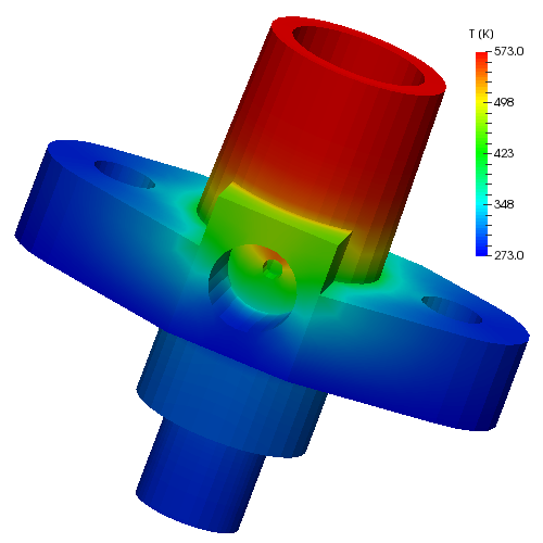
| Conduction + Convection (Conjugate Heat Transfer) |
- chtMultiRegionSimpleFoam (Steady)
- chtMultiRegionFoam (Transient)
| + Radiation |
All the above solvers but laplacianFoam are able to deal with the radiative heat transfer. There are the following five (virtually four) models available in OpenFOAM. Their source code is located in src/thermophysicalModels/radiation/radiationModels and we can see the brief descriptions in the header file of each radiation class.
- P1
|
24 25 26 27 28 29 30 31 32 33 34 |
Class Foam::radiation::P1 Description Works well for combustion applications where optical thickness, tau is large, i.e. tau = a*L > 3 (L = distance between objects) Assumes - all surfaces are diffuse - tends to over predict radiative fluxes from sources/sinks *** SOURCES NOT CURRENTLY INCLUDED *** |
Keywords: optical thickness [2]
- fvDOM (Finite Volume Discrete Ordinates Method)
|
24 25 26 27 28 29 30 31 32 33 34 35 36 37 38 39 40 41 42 43 44 45 46 47 48 49 50 51 52 53 54 55 56 57 58 59 |
Class Foam::radiation::fvDOM Description Finite Volume Discrete Ordinates Method. Solves the RTE equation for n directions in a participating media, not including scatter. Available absorption models: constantAbsorptionEmission greyMeanAbsoprtionEmission wideBandAbsorptionEmission i.e. dictionary \verbatim fvDOMCoeffs { nPhi 4; // azimuthal angles in PI/2 on X-Y. //(from Y to X) nTheta 0; // polar angles in PI (from Z to X-Y plane) convergence 1e-3; // convergence criteria for radiation //iteration maxIter 4; // maximum number of iterations cacheDiv true; // cache the div of the RTE equation. //NOTE: Caching div is "only" accurate if the upwind scheme is used //in div(Ji,Ii_h) } solverFreq 1; // Number of flow iterations per radiation iteration \endverbatim The total number of solid angles is 4*nPhi*nTheta. In 1D the direction of the rays is X (nPhi and nTheta are ignored) In 2D the direction of the rays is on X-Y plane (only nPhi is considered) In 3D (nPhi and nTheta are considered) |
- viewFactor
|
24 25 26 27 28 29 30 31 32 33 34 35 36 37 |
Class Foam::radiation::viewFactor Description View factor radiation model. The system solved is: C q = b where: Cij = deltaij/Ej - (1/Ej - 1)Fij q = heat flux b = A eb - Ho and: eb = sigma*T^4 Ej = emissivity Aij = deltaij - Fij Fij = view factor matrix |
- opaqueSolid
|
24 25 26 27 28 29 30 |
Class Foam::radiation::opaqueSolid Description Radiation for solid opaque solids - does nothing to energy equation source terms (returns zeros) but creates absorptionEmissionModel and scatterModel. |
- none
|
24 25 26 27 28 29 |
Class Foam::radiation::noRadiation Description No radiation - does nothing to energy equation source terms (returns zeros) |
The settings of the radiation models are described in constant/radiationProperties file.
| References |