Many thermal boundary conditions are available in OpenFOAM.
I will upload some basic cases that explain the usage of these boundary conditions.
Source Code
src/TurbulenceModels/compressible/turbulentFluidThermoModels/derivedFvPatchFields/
- convectiveHeatTransfer
It calculates the heat transfer coefficients from the following empirical correlations for forced convection heat transfer:
\begin{eqnarray}
\left\{
\begin{array}{l}
Nu = 0.664 Re^{\frac{1}{2}} Pr^{\frac{1}{3}} \left( Re \lt 5 \times 10^5 \right) \\
Nu = 0.037 Re^{\frac{4}{5}} Pr^{\frac{1}{3}} \left( Re \ge 5 \times 10^5 \right) \tag{1} \label{eq:NuPlate}
\end{array}
\right.
\end{eqnarray}
where \(Nu\) is the Nusselt number, \(Re\) is the Reynolds number and \(Pr\) is the Prandtl number. - externalCoupledTemperature
- externalWallHeatFluxTemperature
This boundary condition can operate in the following two modes:
Mode#1 Specify the heat flux \(q\)
\begin{equation}
-k \frac{T_p – T_b}{\vert \boldsymbol{d} \vert} = q + q_r \tag{2} \label{eq:fixedHeatFlux}
\end{equation}
* \(k\): thermal conductivity
* \(q_r\): radiative heat flux
* \(T_b\): temperature on the boundaryMode#2 Specify the heat transfer coefficient \(h\) and the ambient temperature \(T_a\) (Fig. 1)
\begin{equation}
-k \frac{T_p – T_b}{\vert \boldsymbol{d} \vert} = \frac{T_a – T_b}{R_{th}} + q_r \tag{3} \label{eq:fixedHeatTransferCoeff}
\end{equation}
* \(R_{th}\): total thermal resistance of convective and conductive heat transfer
\begin{equation}
R_{th} = \frac{1}{h} + \sum_{i=1}^{n} \frac{l_i}{k_i} \tag{4} \label{eq:Rth}
\end{equation}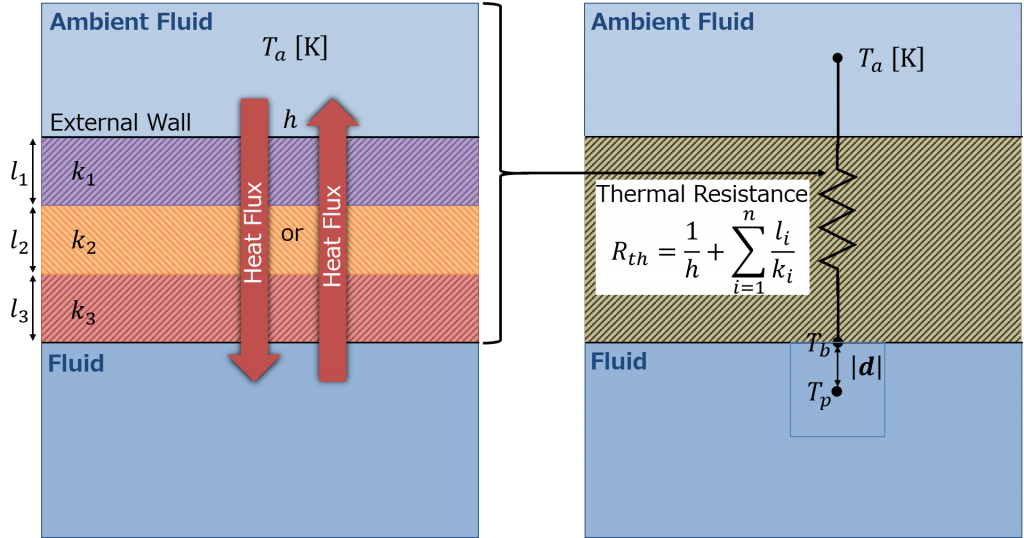
Figure 1 - fixedIncidentRadiation
- lumpedMassWallTemperature
There is a dimensionless quantity called the Biot number, which is defined as
\begin{equation}
Bi = \frac{l/k}{1/h} = \frac{hl}{k}, \tag{5} \label{eq:Biot}
\end{equation}
where \(h\) is the heat transfer coefficient, \(k\) is the thermal conductivity of a solid and \(l\) is the characteristic length of the solid. As the definition in Eq. \eqref{eq:Biot} indicates, it represents the ratio of the internal conduction resistance \(l/k\) and the external convection resistance \(1/h\). If the Biot number is small (\(Bi \ll 1\)), the solid may be treated as a simple lumped mass system of an uniform temperature. This boundary condition calculates the uniform temperature variation \(\Delta T\) on the boundary from the following equation:
\begin{equation}
m c_p \Delta T = Q \Delta t. \tag{6} \label{eq:lumpedmass}
\end{equation}
* \(m\): total mass [kg]
* \(c_p\): specific heat capacity [J/(kg.K)]
* \(Q\): net heat flux on the boundary [W]
* \(\Delta t\): time step [s] - outletMappedUniformInletHeatAddition
- totalFlowRateAdvectiveDiffusive
- wallHeatTransfer
- compressible::thermalBaffle1D
- compressible::turbulentHeatFluxTemperature
- compressible::turbulentTemperatureCoupledBaffleMixed
- compressible::turbulentTemperatureRadCoupledMixed
- compressible::alphatJayatillekeWallFunction
- compressible::alphatPhaseChangeWallFunction
- compressible::alphatWallFunction
Amazing!