This is the second in a series of posts about the computational aeroacoustics and I will try to introduce the very basics of the acoustic wave with some pictures.
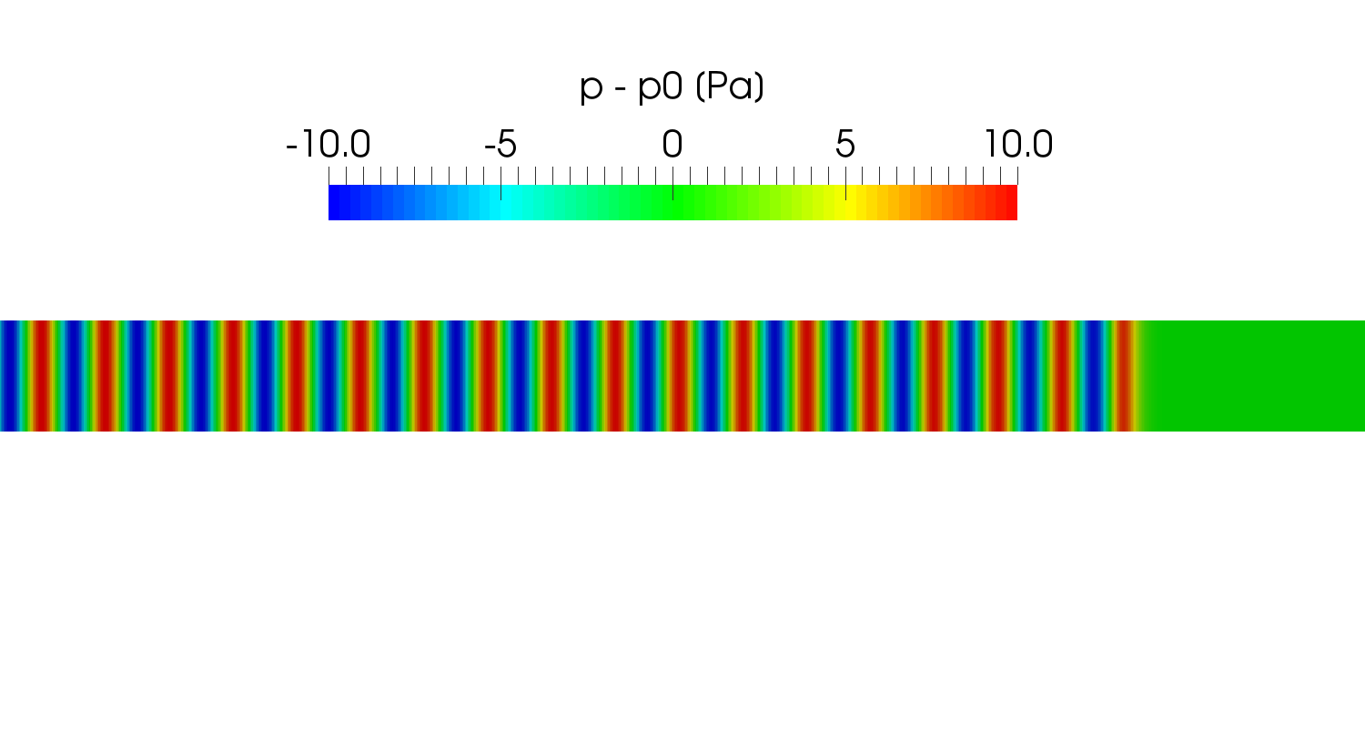
We consider an oscillatory motion with small amplitude in a compressible fluid as shown in the following picture. It shows the distribution of the sound pressure (acoustic pressure) that is defined as the local pressure deviation from the equilibrium pressure \(p_0\) caused by the sound wave propagating from left to right direction.
Since we now consider small oscillations, we can write the local pressure \(p\) and density \(\rho\) in the form
\begin{align}
p &= p_0 + p^{´}, \tag{1a} \label{eq:pressure} \\
\rho &= \rho_0 + \rho^{´}, \tag{1b} \label{eq:density}
\end{align}
where \(p_0\) and \(\rho_0\) are the constant equilibrium pressure and density and \(p^{´}\) and \(\rho^{´}\) are their variations in the sound wave (\(p^{´} \ll p_0, \rho^{´} \ll \rho_0\)), so the above figure is the contour of \(p^{´}\).
We hereafter ignore the fluid viscosity so that only the effect of compressibility is taken into account. Then, the governing equations of the fluid flow is the continuity equation
\begin{align}
\frac{\partial \rho}{\partial t} + \nabla \cdot (\rho \boldsymbol{u}) = 0 \tag{2} \label{eq:continuity}
\end{align}
and the Euler’s equation
\begin{align}
\frac{\partial \boldsymbol{u}}{\partial t} + (\boldsymbol{u} \cdot \nabla)\boldsymbol{u} + \frac{1}{\rho}\nabla p = 0 \tag{3} \label{eq:euler}
\end{align}
where \(\boldsymbol{u}\) is the velocity field. Substituting the eqns. \eqref{eq:pressure} and \eqref{eq:density} into the governing equations and neglecting small quantities of the second order, we get
\begin{align}
\frac{\partial \rho^{´}}{\partial t} + \rho_0 \nabla \cdot \boldsymbol{u} = 0, \tag{4} \label{eq:continuity2}
\end{align}
and
\begin{align}
\frac{\partial \boldsymbol{u}}{\partial t} + \frac{1}{\rho_0} \nabla p^{´} = 0. \tag{5} \label{eq:euler2}
\end{align}
We notice that a sound wave in an ideal fluid is adiabatic and the following relationship holds between the small changes in the pressure and density
\begin{align}
p^{´} = \left(\frac{\partial p}{\partial \rho} \right)_s \rho^{´} \tag{6} \label{eq:adiabatic}
\end{align}
where the subscript s denotes that the partial derivative is taken at constant entropy. Substituting it into \eqref{eq:continuity2}, we get
\begin{align}
\frac{\partial p^{´}}{\partial t} + \rho_0 \left(\frac{\partial p}{\partial \rho} \right)_s \nabla \cdot \boldsymbol{u} = 0. \tag{7} \label{eq:continuity3}
\end{align}
If we introduce the velocity potential \(\boldsymbol{u} = \nabla \phi\), we can derive the relationship between \(p^{´}\) and the potential \(\phi\) from \eqref{eq:euler2}
\begin{align}
p^{´} = -\rho_0 \frac{\partial \phi}{\partial t}. \tag{8} \label{eq:pandphi}
\end{align}
We then obtain the following wave equation from \eqref{eq:continuity3}
\begin{align}
\frac{\partial^2 \phi}{\partial t^2} – c^2 \Delta \phi = 0 \tag{9} \label{eq:waveEqn}
\end{align}
where \(c\) is the speed of sound in an ideal fluid
\begin{align}
c = \sqrt{\left(\frac{\partial p}{\partial \rho} \right)_s}. \tag{10} \label{eq:soundSpeed}
\end{align}
Applying the gradient operator to \eqref{eq:waveEqn}, we find that the each of the three components of the velocity \(\boldsymbol{u}\) satisfies an equation having the same form, and on differentiating \eqref{eq:waveEqn} with respect to time we see that the pressure \(p^{´}\) (and therefore \(\rho^{´}\)) also satisfies the wave equation.
– Landau and Lifshitz, Fluid Mechanics
In a travelling plane wave,
we find
\begin{align}
u_x = \frac{p^{´}}{\rho_0 c}. \tag{11} \label{eq:uxandp}
\end{align}Substituting here from \eqref{eq:adiabatic} \(p^{´} = c^2 \rho^{´}\), we find the relation between the velocity and the density variation:
\begin{align}
u_x = \frac{c \rho^{´}}{\rho_0}. \tag{12} \label{eq:uxandrho}
\end{align}– Landau and Lifshitz, Fluid Mechanics
This book is freely accessible from the link.
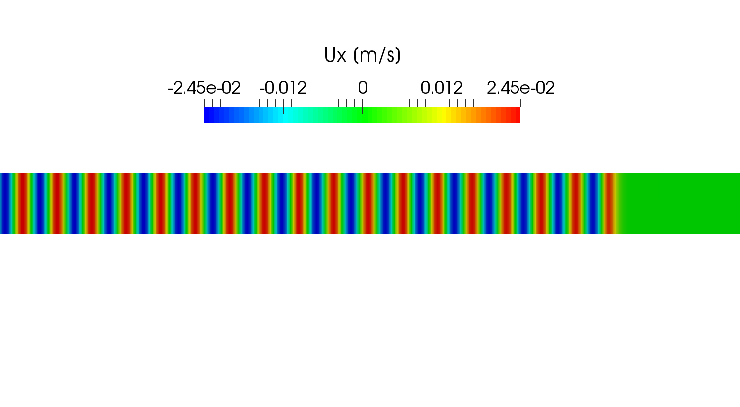
The following picture shows the velocity distribution \(u_x\) calculated using a compressible solver in OpenFOAM at the time corresponding to the pressure variation shown in the above picture. We can calculate the velocity using \eqref{eq:uxandp}
\begin{align}
u_x = \frac{10}{1.2 \times 340} = 0.0245 [m/s]
\end{align}
and it is in good agreement with the result obtained using OpenFOAM.